Dimitris K. Tasoulis, Niall M. Adams, David J. Hand. Institute for .... that depends on both the spatial bandwidth matrix H, and the temporal bandwidth ht.
Unsupervised Clustering In Streaming Data Dimitris K. Tasoulis, Niall M. Adams, David J. Hand Institute for Mathematical Sciences Imperial College London, South Kensington Campus London SW7 2PG, United Kingdom {d.tasoulis,n.adams,d.j.hand}@imperial.ac.uk Abstract Tools for automatically clustering streaming data are becoming increasingly important as data acquisition technology continues to advance. In this paper we present an extension of conventional kernel density clustering to a spatio-temporal setting, and also develop a novel algorithmic scheme for clustering data streams. Experimental results demonstrate both the high efficiency and other benefits of this new approach.
1. Introduction Streaming data presents new challenges to data mining algorithms. These challenges are at least threefold, and arise primarily from the dynamically changing nature of the streams. First, and critical in this area, methods must provide timely results. Second, algorithms must have the capacity to adapt rapidly to changing dynamics of the sequences. Finally, scalability in the number of sequences is becoming increasingly desirable, as data collection technology develops. Density-based methods are an important category of clustering algorithms. These methods partition data into clusters of high density, surrounded by regions of low density. In this paper we propose a density-based approach to data stream clustering that utilises hyperrectangles to discover clusters. Specifically, the proposed approach aims at encapsulating clusters using linear containers in the shape of d-dimensional hyperrectangles. These hyperrectangles are incrementally adjusted to capture the dynamics of changing data streams. The paper proceeds with a presentation of related work in the next Section. In Section 3, we present the extension of kernel density estimation to a spatio-temporal setting. Next, in Section 4 we propose a new clustering method for data streams, and in Section 5, we present experimental results that demonstrate the method’s efficiency. The paper ends with concluding remarks in Section 6.
2. Related Work Most clustering methods cannot be used for streaming data since they rely on the assumption that the data are available in a permanent memory structure, from which global information can be obtained at any time. Incremental extensions have been proposed for batch algorithms [10], that focus on applications of periodically updated databases. More recent approaches have focused precisely on the streaming data model. The CluStream algorithm proposed in [2], assumes the behaviour of the data stream may evolve over time, but uses a predefined constant number of microclusters to determine the clustering results. The interesting concept of projected clustering was introduced in [3], but it is hindered by the inability to discover clusters of arbitrary orientation. A k-means clustering model for data streams was proposed in [5]. Most recently, [4] developed the HPSTREAM algorithm, by extending the GDBSCAN algorithm to streaming data. The extension used microclusters [3] to maintain a model of the data density in memory. Finally, [11] proposed a a density estimation method that adapts to the available computation resource. A subsequent clustering algorithm is required to determine the final grouping.
3. Temporal Kernel Density Estimation Density estimation [8] is an established non-parametric approach to cluster analysis. The rationale behind density estimation is that the data space can be regarded as the empirical probability density function (pdf) of the data. In this sense local maxima of the pdf can be thought to correspond to centres of clusters. Kernel density estimation is one of the most popular density estimation methods [8]. Let a data set X = {x1 , . . . , xn }, where xj is a data vector in the ddimensional Euclidean space Rd . The multivariate kernel
density estimate fˆH (x), computed at point x is given by: n � � 1� fˆH (x) = KH H −1 (x − xi ) , n i=1
(1)
where H is the bandwidth matrix and KH () : Rd �→ R is a kernel function. The bandwidth matrix controls the variance of the kernel function and serves as a smoothing parameter. The first attempt to extend kernel density estimation to the temporal domain was [1]. In this framework the data set is assumed to have the following spatio-temporal form: X � = {{x1 , t1 }, . . . , {xn , tn }}, where xj is a data vector in the d-dimensional Euclidean space Rd , and tj represents the timestamp at which xj arrives. Thus, a typical streaming data point is {xj , tj }. Additionally, the fading function Tht (t), associates a weight with each timestamp, that decreases with time. The parameter ht , represents the forgetting factor of previous data. In this case a temporal kernel can be defined as follows: � (X, t) = Tht (t)KH (H −1 X), KH,h t
(2)
that depends on both the spatial bandwidth matrix H, and the temporal bandwidth ht . The kernel density estimate for a specific timestamp t0 , at the location x, is defined as: � −1 � �n � (x − xi )), (t0 − ti ) i=1 KH,ht (H ˆ fH (x, to ) = �t0 t=0 Tht (t0 − t) (3) Note also that t � t0 , since we do not have any information for future data.
4. Temporal Clustering though Windows In the context of streaming data, retaining historical data to use Eq. 2 is at best impractical, and at worst impossible. Thus it is essential to reduce the storage overhead by reducing the amount of data retained. Using windows to determine clusters is a plausible technique that allows fast processing, and at the same time is able to produce high quality results [9]. For a spatio-temporal dataset X � with a spatio-temporal form of the Epanechnikov kernel, � (d+2)Tht (t)(1−�H −1 c�2 ) if �H −1 c� < 1 � 2cKH ,d KH,ht (c, t) = 0 otherwise (4) with a window defined as the set of points that are included in the support of the kernel (�H −1 c� < 1): Definition 4.1. A spatio-temporal window W for the spatio-temporal dataset X � , is defined by a diagonal bandwidth matrix, H = diag(h1 , . . . , hd ),
where hi ∈ Rd,+ , i = 1, . . . d, and a point c ∈� Rd (centre of the window) � such that: W = {x, t} ∈ X : �H −1 (c − x)�∞ < 1 . Note that in the above definition we employ the � · �∞ norm, since this allows fast computation and, as we demonstrate later, provides an intuitive way of determining the bandwidth matrix H. Our proposed clustering scheme operates by maintaining a list of windows in memory, such that windows are incrementally adjusted with the arrival of new data to best suit the underlying clustering structure. Specifically, it uses two fundamental procedures “movement”, and “enlargement-contraction”. These two procedures are analysed in the following paragraphs. Movements In the present setting, the movement procedure incrementally re-centers windows every time a new streaming data point arrives. Windows are re-centered to the mean of the points they include at time t0 , mW,t0 , in a manner that also depends on the points’ timestamps: � −1 � � � (x − xi )), (t0 − ti ) {xi ,ti }∈W KH,ht (H � mW,t0 = . {xi ,ti }∈W Tht (t0 − ti ) (5) The denominator in this fraction actually represents a measure of the total weight of the window. Define this weight as � |W |t0 = Tht (t0 − ti ). (6) {xi ,ti }∈W
Moreover, denote the nominator of Eq.5 as: � � −1 � � (H (x − xi )), (t0 − ti ) . KH,h CW,t0 = t {xi ,ti }∈W
(7) Enlargement-Contraction Using windows to enclose clusters allows the iterative selection of the diagonal elements of the bandwidth matrix, that relate to the scales of the different streams. In the batch case this operation can be performed if the windows are initialised with small values in the bandwidth matrix, and are subsequently iteratively enlarged as long as this increases the value of the kernel density estimate of the window. However, approximations for the window bandwidth in an evolving spatio-temporal setting are complicated by the case of shrinking clusters. To address this, for each co-ordinate j of a window consider the following quantities: � Tht (t0 − ti ), (8) I|W |t0 ,j = {xi ,ti }∈W :
O|W |t0 ,j
=
�c−xi,j �∞ hj
�
�c−xi,j �∞ {xi ,ti }∈W : hj
�θe
Tht (t0 − ti ), (9) >θe
where hj is the jth diagonal element of the diagonal bandwidth matrix H, and 0 < θe < 1, is a user defined parameter. An example of a two-dimensional dataset is demonstrated in Figure 1, where only the unfilled dots are used to compute the value of O|W |t0 ,1 , while the filled dots are used to compute O|W |t0 ,1 . Iterative contractions and enx2
θe h 1
W
I|W |t0 ,1 O|W |t0 ,1 h1 x1
Figure 1. An example of the difference between I|W |t0 ,j and O|W |t0 ,j .
largements of the windows is controlled by specifying rules for the fraction of these values. If it holds that for any coordinate j of the window:
O|W |t
,j
I|W |t
,j
0
0
> 1.0 + θe , then the win-
dow is enlarged through the equation hj ← hj + hj × θe . Similarly if
I|W |t
0
O|W |t
,j
0
,j
> 1.0 + θe , then the window is con-
tracted through the equation hj ← hj − hj × θe . The Algorithm The proposed clustering algorithm maintains a set of windows that define the clustering result at each time point. Whenever such a clustering needs to be produced for a set of streaming data points, only their inclusion in the maintained windows needs to be examined. Let us assume an exponential fading function of the form Tht (t) = 2−ht t with ht > 0. Such functions are commonly used in temporal applications. Smaller values of ht give more importance to historical data compared to data that have just arrived. The algorithm is initialised with an empty list of windows, L. Each time a new streaming data point x arrives, we interrogate the window list. If no window in the list includes the point, a new window, centered on this point, is created and added to L. This window, W , has an initial user defined size α, and its weight variables are initialised as I|W |t0 ,j = 1, O|W |t0 ,j = 1, |W |t0 = 1, for j = 1, . . . , d. If there are windows in L that include a new streaming data point, then their centres and weights are updated through the equations (5),(6),(8), and (9). At first glance, this would mean that all the previous data points, as well as their timestamps should be available. However this is not necessary since they can be maintained incrementally. Let us suppose that for window W , no points arrived that were included in W from time point t1 , until the current time tc Then the corresponding values can be updated as
follows: |W |tc
= 2−λ(tc −t1 ) |W |t1 + 1
CW,tc
= 2−λ(tc −t1 ) |W |t1 � � +KH (H −1 (CW,t1 − x)) CW,tc = |W |tc
mW,tc
(10) (11) (12)
Moreover for each coordinate j, depending on the values of the respective coordinates xj of x, the values of I|W |tc ,j , and O|W |tc ,j , can be incrementally updated in a analogous manner: I|W |tc ,j O|W |tc ,j
= =
2−λ(tc −t1 ) I|W |t1 ,j + 1 2
−λ(tc −t1 )
O|W |tc ,j + 1
(13) (14)
Periodically, every T time steps, we can check the list L for windows with very small weight (lower than a minimum value wmin ), and delete them from the list since they correspond to areas of the data space that are either very old compared to the defined time horizon, or just contain outlier points. A high level description of the WSTREAM algorithm follows: Algorithm WSTREAM (L,θe ,T ,wmin) for each point arrival x, tx do for each window Wl ∈ L of centre cl , and bandwidth matrix Hl , that satisfies �Hl−1 (cl − x)�∞ < 1 do update |Wl |tx , CWl ,tx , and mWl ,tx through Eqs.(10),(11) and (12). for each coordinate j, j = 1, . . . d, do �c −x � if l.j hji,j ∞ � θe then update I|Wl |tx ,j through Eq.(13), else update O|Wl |tx ,j through Eq.(14). if
O|Wl |t ,j x I|Wl |t ,j
> 1.0 + θe , then
I|Wl |t ,j x O|Wl |t ,j
> 1.0 + θe , then
x
set hj ← hj + hj ∗ θe . if
x
set hj ← hj − hj ∗ θe . if tx mod T = 0, remove from L, windows with weight lower than wmin . The WSTREAM algorithm maintains a list of windows that captures the cluster structure of the data. However, this structure is only realised for a specific set of streaming data points. To define a cluster structure for such a point set, we simply check the point’s participation in the set of windows. In this way it is also possible to approximate the cluster number. During this cluster defining operation the number of streaming data points that lie in the intersection of each pair of overlapping windows is computed. Next, the proportion of this number to the total number of streaming data points included in each window is calculated. If
this proportion exceeds a user defined threshold, θs , the two windows are considered to be identical and we disregard the window containing the fewer points. Otherwise, if that proportion exceeds a second user defined threshold, θm , the windows are considered to have captured portions of the same cluster and are merged. An example of this operation is exhibited in Fig. 2; the extent of overlap of windows W1 and W2 exceeds the θs threshold and W1 is deleted. On the other hand, windows W3 and W4 are considered both to belong to the same cluster. Finally, windows W5 and W6 , are considered to capture two different clusters. As already de(a)
(b) W1
(c)
W3
W5
W2 W4
W6
Figure 2. Determining the number of clusters.
scribed, the WSTREAM algorithm needs only a single pass over the dataset, which satisfies the constraints imposed by streaming data. The memory requirements of the algorithm strongly depend on the complexity of the underlying cluster structure. This is because a cluster is defined by at least one window. To this end, as the number of clusters grows more memory is required to keep track of their structure. Moreover, if the clusters have a non-convex shape then more than one window is required to capture their structure [9].
5. Experimental Results To test the the efficiency of the WSTREAM algorithm we first employ the Forest CoverType real world data set, obtained from the UCI machine learning repository [7]. This data set, DsetForest , is comprised of 581012 observations characterised using 54 attributes, where each observation is labeled in one of seven forest cover classes. We retain the 10 numerical attributes. To measure clustering efficiency we employed the cluster purity measure P , [3, 4], Pk
|Di |
defined as: P = i=1k |Ni | , where |Di | denotes the number of points with the dominant class label in cluster i, |Ni | the total number of points in cluster i, and k, the number of clusters. Intuitively, this measures the purity of the clusters with respect to the true cluster (class) labels that are known for our data sets. In Fig. 3(a), we exhibit the purity of the clustering result obtained in the last 2000 points for various time points of the data stream. Note that purity is never lower than 80%. Additionally, to examine sensitivity to various parameters, at time point 20000, we examine the purity of the clustering result on the last 2000 records, obtained for different values of the parameters a (initial size of the window), and θe (enlarge-contract parameter). Fig.3(b) shows
that for α > 3 very high purity results are obtained, while for values over 14 the results deteriorate. Finally, Fig.3(c) demonstrates the effect of θe . This parameter exhibits similar behaviour, in that a wide range of values result in good performance. The choice of the temporal bandwidth parameter λ did not prove to be crucial in obtaining good results so we exclude it from the plots. The final dataset, DsetKDD , was obtained from the KDD 1999 intrusion detection contest [6]. We took the first 100,000 objects and the 37 numerical attributes. 77, 888 of these objects correspond to “normal connections” and 22, 112 correspond to “Denial of Service” (DoS) attacks. Treating this as streaming data, and examining the clustering result of the last 100, 200, and 1, 000, points at various time points between 10, 000 and 100, 000, we never observed a clustering purity of less than 0.98. Using the above sensitivity analysis of the parameters, we used the values 5, 0.01, 0.1, for the parameters a, λ and θe , respectively. Comparisons to Other Algorithms In this work we have used the same datasets as similar works, and this greatly facilitates comparison of our proposed approach to related algorithms. Specifically, both DsetKDD , and DsetForest , have been used in assessment of HPSTREAM [3] and DENSTREAM [4]. We have measured clustering efficiency in a similar manner, and our results yield superior purity to these other approaches. To compare the three algorithms we constructed a series of artificial datasets Dset3 , by drawing 20,000 random points from a mixture of 5-dimensional spherical Gaussian distributions. The number of Gaussians varied between 2 and 100, in order to measure the scalability of the algorithms with respect to the number of clusters in the data. Similarly, a series of artificial datasets, Dset4 , was constructed in a similar manner, with the number of Gaussians fixed at 5, and the dimensionality varied between 2 and 20. The mean of all the Gaussians was uniformly scattered in the interval [0, 2000] for each coordinate, and the variance along each dimension was a uniformly chosen number in the interval [0.5, 5]. The required processing time for a 2.8GHz Pentium 4 personal computer with 1GB of memory was measured for both series of datasets; Dset3 , and Dset4 . we used the suggestions in [3, 4] to set the parameters of HPSTREAM and DENSTREAM. For HPSTREAM we set the number of fading cluster structures as twice the true cluster number in all cases. For DENSTREAM, the � parameter was set to 2.0, that is half the size of the largest possible covariance. The results are presented in Figs. 4(a) and (b). Since there is some randomness involved, all the experiments were performed 10 times. In the figures the mean of these experiments is displayed, along with vertical lines that depict the variation of the observed times. Although HPSTREAM is a projected clustering algorithm, additional
(b)
(c) 94
94
96
92
92
94 92 90
Purity (%)
98
Purity (%)
Purity (%)
(a)
90 88 86
90 88 86
88 84
84
84
82
82
82
80
86
0
50000 100000 150000 200000 250000 300000 350000 400000
80 0
time
2
4
6
8
10
α
12
14
16
18
20
0
0.1
0.2
0.3
θe
0.4
0.5
0.6
0.7
Processing Time
Figure 3. Results for the DsetForest , and different parameter settings. (a)
clustering community. It is a considerable challenge to extend such clustering methods to the spatio-temporal form of streaming data. Our proposed algorithmic scheme appears able to capture evolving cluster dynamics and provide both efficient and meaningful results.
2.5 HPSTREAM DENSTREAM 2
WSTREAM
1.5
1
References
0.5
0
Processing Time
10
20
30
40
50
60
70
80
90
100
Number of Clusters
(b)
1.6 HPSTREAM 1.4
DENSTREAM
1.2
WSTREAM
1 0.8 0.6 0.4 0.2 0 2
4
6
8
10
12
14
16
18
20
Dimension Figure 4. Processing time in seconds for the series of datasets Dset3 and Dset4 .
computational resources are required, making it the most time consuming of the three. On the other hand, the increasing number of dimensions introduce less additional computational burden for DENSTREAM and WSTREAM. In the case of increasing number of clusters, both DENSTREAM and WSTREAM exhibit very similar performance. However, note that all the algorithms have less than linear increase in computation time with respect to both the dimensions and the number of clusters.
6. Concluding Remarks Kernel density estimation is an established nonparametric technique that has been successfully used by the
[1] C. Aggarwal. A framework for diagnosing changes in evolving data streams, 2003. [2] C. Aggarwal, J. Han, J. Wang, and P. Yu. A framework for clustering evolving data streams. In 9th VLDB conference, 2003. [3] C. Aggarwal, J. Han, J. Wang, and P. Yu. A framework for projected clustering high dimensional data streams. In 10th VLDB conference, 2004. [4] F. Cao, M. Ester, W. Qian, and A. Zhou. Density-based clustering over an evolving data stream with noise. In 2006 SIAM Conference on Data Mining, 2006. to appear. [5] P. Domingos and G. Hulten. A general method for scaling up machine learning algorithms and its application to clustering. In Proc. 18th International Conf. on Machine Learning, pages 106–113. Morgan Kaufmann, San Francisco, CA, 2001. [6] KDD. Cup data a.v.I http://kdd.ics.uci.edu/ databases/kddcup99/kddcup99.html, 1999. [7] D. Newman, S. Hettich, C. Blake, and C. Merz. UCI repository of machine learning databases, 1998. [8] B. Silverman. Density Estimation for Statistics and Data Analysis. Monographs on Statistics and Applied Probability. Chapman and Hall, 1986. [9] D. Tasoulis and M. Vrahatis. Novel approaches to unsupervised clustering through the k-windows algorithm. In S. Sirmakessis, editor, Knowledge Mining, volume 185 of Studies in Fuzziness and Soft Computing, pages 51–78. SpringerVerlag, 2005. [10] D. Tasoulis and M. Vrahatis. Unsupervised clustering on dynamic databases. Pattern Recognition Letters, 26(13):2116– 2127, 2005. [11] W. Zhu, J. Pei, J. Yin, and Y. Xie. Granularity adaptive density estimation and on-demand clustering of concept-drifting data streams. In 8th International Conference on Data Warehousing and Knowledge Discovery (DaWaK’06), Krakow, Poland, 2006.