autoencoder (known as VAE) and the Gaussian Mixture variational autoencoder (called ..... space that aims to capture the multimodal nature of the input data.
Degree in Telecommunication Technologies Engineering 2017-2018
Bachelor Thesis
Unsupervised Deep Learning Research and Implementation of Variational Autoencoders
Pablo Sánchez Martín Supervised by Pablo Martínez Olmos Leganés, June 2018
This work is licensed under a Creative Commons Attribution-Noncommercial-NoDerivative License.
Abstract Generative models have been one of the major research fields in unsupervised deep learning during the last years. They are achieving promising results in learning the distribution of multidimensional variables as well as in finding meaningful hidden representations in data. The aim of this thesis is to gain a sound understanding of generative models through a profound study of one of the most promising and widely used generative models family, the variational autoencoders. In particular, the performance of the standard variational autoencoder (known as VAE) and the Gaussian Mixture variational autoencoder (called GMVAE) is assessed. First, the mathematical and probabilistic basis of both models is presented. Then, the models are implemented in Python using the Tensorflow framework. The source code is freely available and documented in a personal GitHub repository created for this thesis. Later, the performance of the implemented models is appraised in terms of generative capabilities and interpretability of the hidden representation of the inputs. Two real datasets are used during the experiments, the MNIST and "Frey faces". Results show the models implemented work correctly, and they also show the GMVAE outweighs the performance of the standard VAE, as expected. Keywords: deep learning, generative model, variational autoencoder, Monte Carlo simulation, latent variable, KL divergence, ELBO.
iii
ACKNOWLEDGEMENTS To start with, I would like to thank my family, for being completely supportive throughout the time I have been conducting this thesis and the degree. I would like to thank specially my parents for helping me on a daily basis, both on the good and bad times, for teaching me important principles such as perseverance and basically, for everything they do. I would also like to thank my university colleagues with which I have shared unforgettable memories during the last years. Last but not least, I would like to thank my supervisor Pablo M. Olmos. I am extremely grateful to him for the time he has invested in teaching me everything this thesis required, in resolving any issue that arose and for being such a good mentor. Thank you all for your trust and support.
v
CONTENTS 1. INTRODUCTION. . . . . . . . . . . . . . . . . . . . . . . . . . . . . . . . . . . .
1
1.1. Statement of Purpose . . . . . . . . . . . . . . . . . . . . . . . . . . . . . . . .
1
1.2. Requirements . . . . . . . . . . . . . . . . . . . . . . . . . . . . . . . . . . . . .
2
1.2.1. Datasets . . . . . . . . . . . . . . . . . . . . . . . . . . . . . . . . . . . . . .
2
1.2.2. Programming Framework . . . . . . . . . . . . . . . . . . . . . . . . . . . .
3
1.2.3. GPU Power . . . . . . . . . . . . . . . . . . . . . . . . . . . . . . . . . . . .
3
1.3. Regulatory Framework . . . . . . . . . . . . . . . . . . . . . . . . . . . . . . .
4
1.3.1. Legislation . . . . . . . . . . . . . . . . . . . . . . . . . . . . . . . . . . . .
4
1.4. Work Plan . . . . . . . . . . . . . . . . . . . . . . . . . . . . . . . . . . . . . . .
5
1.5. Organization . . . . . . . . . . . . . . . . . . . . . . . . . . . . . . . . . . . . .
5
2. BACKGROUND . . . . . . . . . . . . . . . . . . . . . . . . . . . . . . . . . . . .
7
2.1. Overview of Generative Models . . . . . . . . . . . . . . . . . . . . . . . . . .
7
2.1.1. Explicit Density Models . . . . . . . . . . . . . . . . . . . . . . . . . . . . .
8
2.1.2. Implicit Density Models . . . . . . . . . . . . . . . . . . . . . . . . . . . . .
8
2.2. Probabilistic PCA . . . . . . . . . . . . . . . . . . . . . . . . . . . . . . . . . .
9
2.3. Neural Networks . . . . . . . . . . . . . . . . . . . . . . . . . . . . . . . . . . . 11 2.3.1. Convolutional Neural Networks . . . . . . . . . . . . . . . . . . . . . . . . 12 3. VARIATIONAL AUTOENCODER . . . . . . . . . . . . . . . . . . . . . . . . . . 14 3.1. Overview . . . . . . . . . . . . . . . . . . . . . . . . . . . . . . . . . . . . . . . 14 3.2. Objective . . . . . . . . . . . . . . . . . . . . . . . . . . . . . . . . . . . . . . . 16 3.2.1. Dealing with the Integral over z . . . . . . . . . . . . . . . . . . . . . . . . 16 3.2.2. Inference Network: qϕ (z|x) . . . . . . . . . . . . . . . . . . . . . . . . . . . 17 3.2.3. KL Divergence . . . . . . . . . . . . . . . . . . . . . . . . . . . . . . . . . . 17 3.2.4. Core Equation . . . . . . . . . . . . . . . . . . . . . . . . . . . . . . . . . . 18 3.2.5. ELBO Optimization . . . . . . . . . . . . . . . . . . . . . . . . . . . . . . . 19 3.2.6. Reparameterization Trick . . . . . . . . . . . . . . . . . . . . . . . . . . . . 21 3.3. Sampling . . . . . . . . . . . . . . . . . . . . . . . . . . . . . . . . . . . . . . . 21
vii
4. GAUSISIAN MIXTURE VARIATIONAL AUTOENCODER . . . . . . . . . . . 22 4.1. Introduction. . . . . . . . . . . . . . . . . . . . . . . . . . . . . . . . . . . . . . 22 4.2. Overview . . . . . . . . . . . . . . . . . . . . . . . . . . . . . . . . . . . . . . . 22 4.3. Defining z directly as a GMM . . . . . . . . . . . . . . . . . . . . . . . . . . . 23 4.4. Optimization Function . . . . . . . . . . . . . . . . . . . . . . . . . . . . . . . . 23 4.4.1. Reconstruction Term . . . . . . . . . . . . . . . . . . . . . . . . . . . . . . . 25 4.4.2. Conditional prior term . . . . . . . . . . . . . . . . . . . . . . . . . . . . . . 25 4.4.3. W-prior term . . . . . . . . . . . . . . . . . . . . . . . . . . . . . . . . . . . 26 4.4.4. Y-prior term. . . . . . . . . . . . . . . . . . . . . . . . . . . . . . . . . . . . 26 4.4.5. ELBO Equation . . . . . . . . . . . . . . . . . . . . . . . . . . . . . . . . . 26 4.5. Reparameterization Trick . . . . . . . . . . . . . . . . . . . . . . . . . . . . . . 27 4.6. Sampling . . . . . . . . . . . . . . . . . . . . . . . . . . . . . . . . . . . . . . . 27 5. METHODOLOGY . . . . . . . . . . . . . . . . . . . . . . . . . . . . . . . . . . . 28 5.1. Objective . . . . . . . . . . . . . . . . . . . . . . . . . . . . . . . . . . . . . . . 28 5.2. Prepare Data . . . . . . . . . . . . . . . . . . . . . . . . . . . . . . . . . . . . . 28 5.3. Model Architecture . . . . . . . . . . . . . . . . . . . . . . . . . . . . . . . . . 29 5.4. Definition of hyperparameters . . . . . . . . . . . . . . . . . . . . . . . . . . . 29 5.5. Experimental Setup . . . . . . . . . . . . . . . . . . . . . . . . . . . . . . . . . 30 5.6. GMAVE numerical stability. . . . . . . . . . . . . . . . . . . . . . . . . . . . . 32 5.6.1. Approximation of pβ (y j = 1|w, z) . . . . . . . . . . . . . . . . . . . . . . . . 32 5.6.2. Output restrictions . . . . . . . . . . . . . . . . . . . . . . . . . . . . . . . . 33 5.7. Motivate clustering behaviour. . . . . . . . . . . . . . . . . . . . . . . . . . . . 34 5.8. Metrics . . . . . . . . . . . . . . . . . . . . . . . . . . . . . . . . . . . . . . . . 34 5.9. Visualization of results. . . . . . . . . . . . . . . . . . . . . . . . . . . . . . . . 35 6. RESULTS . . . . . . . . . . . . . . . . . . . . . . . . . . . . . . . . . . . . . . . . 37 6.1. Initial considerations . . . . . . . . . . . . . . . . . . . . . . . . . . . . . . . . . 37 6.2. Experiment 1: VAE . . . . . . . . . . . . . . . . . . . . . . . . . . . . . . . . . 37 6.3. Experiment 2: Understanding the latent variables of GMVAE. . . . . . . . . . 39 6.4. Experiment 3: Comparison between GMVAE and VAE . . . . . . . . . . . . . 40 6.5. Experiment 4: Performance evaluation with corrupted input. . . . . . . . . . . 42 6.6. Experiment 5: Convolutional architecture . . . . . . . . . . . . . . . . . . . . . 43 viii
7. SOCIO-ECONOMIC ENVIRONMENT . . . . . . . . . . . . . . . . . . . . . . . 46 7.1. Budget. . . . . . . . . . . . . . . . . . . . . . . . . . . . . . . . . . . . . . . . . 46 7.2. Practical Applications . . . . . . . . . . . . . . . . . . . . . . . . . . . . . . . . 47 8. CONCLUSIONS . . . . . . . . . . . . . . . . . . . . . . . . . . . . . . . . . . . . 49 8.1. Conclusions. . . . . . . . . . . . . . . . . . . . . . . . . . . . . . . . . . . . . . 49 8.2. Future work . . . . . . . . . . . . . . . . . . . . . . . . . . . . . . . . . . . . . . 50 A. VAE LOSS RESULTS . . . . . . . . . . . . . . . . . . . . . . . . . . . . . . . . . 51 B. GENERATED SAMPLES . . . . . . . . . . . . . . . . . . . . . . . . . . . . . . . 52 C. KL DIVERGENCE OF GMM. . . . . . . . . . . . . . . . . . . . . . . . . . . . . 53 D. GMVAE OBJECTIVE FUNCTION DERIVATIONS. . . . . . . . . . . . . . . . 54 D.1. Conditional prior term. . . . . . . . . . . . . . . . . . . . . . . . . . . . . . . . 54 D.2. W-prior term . . . . . . . . . . . . . . . . . . . . . . . . . . . . . . . . . . . . . 55 D.3. Y-prior term . . . . . . . . . . . . . . . . . . . . . . . . . . . . . . . . . . . . . 55 BIBLIOGRAPHY. . . . . . . . . . . . . . . . . . . . . . . . . . . . . . . . . . . . . . 57
ix
LIST OF FIGURES
1.1
Several samples from the MNIST dataset. . . . . . . . . . . . . . . . . .
2
1.2
Several samples from Frey faces dataset. . . . . . . . . . . . . . . . . . .
3
2.1
Taxonomy of generative models based on maximum likelihood. Extracted from [11]. . . . . . . . . . . . . . . . . . . . . . . . . . . . . . . . . . .
8
2.2
PCA generative model. Extracted from [18]. . . . . . . . . . . . . . . . .
10
2.3
Mathematical model of a simple artificial neuron. . . . . . . . . . . . . .
11
2.4
Several activation functions. . . . . . . . . . . . . . . . . . . . . . . . .
12
2.5
Edge detector kernel. Extracted from [26]. . . . . . . . . . . . . . . . . .
13
2.6
Simple CNN Architecture. . . . . . . . . . . . . . . . . . . . . . . . . .
13
3.1
Probabilistic view of VAE. Extracted from [29]. . . . . . . . . . . . . . .
15
3.2
Graphical models for the VAE showing the generative model (left) and the inference model (right). . . . . . . . . . . . . . . . . . . . . . . . . .
15
Graphical models for the GMVAE showing the generative model (left) and the inference model (right). . . . . . . . . . . . . . . . . . . . . . . .
22
5.1
Data diagram. . . . . . . . . . . . . . . . . . . . . . . . . . . . . . . . .
28
6.1
Example of good clustering but poor generation result. . . . . . . . . . .
38
6.2
Example of poor clustering but good generation result. . . . . . . . . . .
39
6.3
Examples of PCA latent space representation and reconstruction varying dim z. . . . . . . . . . . . . . . . . . . . . . . . . . . . . . . . . . . . .
39
6.4
Scatter plot of variable w.
. . . . . . . . . . . . . . . . . . . . . . . . .
40
6.5
Scatter plot of variable z. . . . . . . . . . . . . . . . . . . . . . . . . . .
40
6.6
Example of bad clustering but good generation result. . . . . . . . . . . .
41
6.7
Example of good clustering and good generation result. . . . . . . . . . .
42
6.8
Reconstruction without noise. . . . . . . . . . . . . . . . . . . . . . . .
43
6.9
Reconstruction with uniform noise. . . . . . . . . . . . . . . . . . . . . .
43
6.10 Reconstruction with dropout noise. . . . . . . . . . . . . . . . . . . . . .
43
6.11 Example of results using GMVAE convolutional architecture on MNIST. .
44
4.1
xi
6.12 Example of results using VAE convolutional architecture on MNIST. Model (a) and (b) with dim z = 2 and model (c) and (d) with dim z = 10. . . . . . 45 6.13 Example of results using GMVAE’s convolutional architecture on FREY dataset. . . . . . . . . . . . . . . . . . . . . . . . . . . . . . . . . . . .
45
B.1 Low quality generated samples with different VAE configurations. . . . .
52
xii
LIST OF TABLES
1.1
Work packages. . . . . . . . . . . . . . . . . . . . . . . . . . . . . . . .
5
5.1
VAE architectures . . . . . . . . . . . . . . . . . . . . . . . . . . . . . .
29
5.2
GMVAE architectures . . . . . . . . . . . . . . . . . . . . . . . . . . . .
29
5.3
Definition of hyperparameters. . . . . . . . . . . . . . . . . . . . . . . .
30
5.4
Experiment 1 Hyper-Parameters. . . . . . . . . . . . . . . . . . . . . . .
31
5.5
Experiment 2 Hyper-Parameters. . . . . . . . . . . . . . . . . . . . . . .
31
5.6
Experiment 5 Hyper-Parameters. . . . . . . . . . . . . . . . . . . . . . .
32
5.7
Metrics selected. . . . . . . . . . . . . . . . . . . . . . . . . . . . . . .
35
6.1
Loss results of the best clustering configurations. Ordered by ValidLoss. .
38
6.2
Loss results of the best generative configurations. Ordered by KLloss. . .
38
6.3
Best clustering configurations of VAE in GMVAE. Ordered by CondPrior.
41
6.4
The best generative configurations of VAE in GMVAE. Ordered by CondPrior. . . . . . . . . . . . . . . . . . . . . . . . . . . . . . . . . . . . . .
41
6.5
Loglikelihood results. . . . . . . . . . . . . . . . . . . . . . . . . . . . .
43
6.6
GMVAE training result. . . . . . . . . . . . . . . . . . . . . . . . . . . .
44
6.7
VAE training result. . . . . . . . . . . . . . . . . . . . . . . . . . . . . .
44
7.1
Detailed budget. . . . . . . . . . . . . . . . . . . . . . . . . . . . . . . .
47
7.2
Practical applications. . . . . . . . . . . . . . . . . . . . . . . . . . . . .
48
xiv
1. INTRODUCTION This chapter presents the project in brief. It contains the motivation and objectives of this thesis, the regulatory framework related to the project, the requirements, the activities undertaken and the overall structure of the document. 1.1. Statement of Purpose Neural networks have existed since the definition of the Perceptron in 1958 [1]. However, they did not become popular until the appearance of backpropagation in the late 80s [2]. Latest advances in distributed computing, specialized hardware and an exponential growth in the amount of data created, have enabled to train extremely complex neural networks with large number of layers and parameters. The discipline that studies this type of networks is known as Deep Learning and it is achieving state-of-the-art results in many difficult problems such as speech recognition [3], object detection [4], text generation [5] and recently in data generation. A generative model is a kind of unsupervised learning model that aims to learn any type of data distribution and it has the potential to unveil underlying structure in the data. Generative models have recently emerged as a revolution in deep learning with many applications in a wide-ranging variety of fields such as medicine, art, gaming or selfdriving. Deep learning, and specially generative models, is evolving so fast that it is difficult to keep up with the latest developments. For these reasons, the purpose of this work is to serve as a sound introduction to deep learning generative models. To achieve this goal, the variational autoencoder model or VAE, one of the most widely used generative models, is studied in detail and compared to one of its variations: the Gaussian Mixture VAE. The implementation of the GMVAE will be based on [6] with some modifications proposed in this work. So the main objective of this bachelor thesis can be expanded as follows: 1. Study in detail the mathematical and probabilistic basis of the variational autoencoders. 2. Explore dimesionality reduction algorithms. 3. Master Tensorflow, a widely used deep learning library for python. 4. Implement the VAE and GMVAE models using different architectures. 5. Compare and evaluate the algorithms implemented for different datasets.
1
As it will be seen further on, the GMVAE describes a two level hierarchical latent space that aims to capture the multimodal nature of the input data. Due to this, the hypothesis of this thesis is that the GMVAE model improves the generative and clustering capabilities of the standard VAE. Experiments will be conducted to test this hypothesis. 1.2. Requirements The first part of this thesis is purely theoretical. In the second part, the following tools are required for the implementation of the models: datasets, programming framework and GPU power. 1.2.1. Datasets The datasets used for this thesis are the MNIST and "Frey faces" (or FREY) datasets, both publicly available. They consist of images with dimension D x that represents the number of pixels: MNIST: D x = 28x28 = 784 FREY: D x = 20x28 = 560 MNIST Dataset The MNIST database [7] is a labeled collection of gray-scale handwritten digits distributed by Yann Lecun’s website. Each image is formed by 28x28 size-normalized pixels. The MNIST database is often used to assess performance of algorithms in research. There are functions available to prepare the dataset so there is no need to write code about preprocessing or formatting.
(a) Label: 2
(b) Label: 3
(c) Label: 8
Fig. 1.1. Several samples from the MNIST dataset.
2
FREY Dataset The "Fray faces" or FREY dataset [8] consists of 1965 images with 20x28 pixels of Brendan’s face taken from sequential frames of a video. Although this is an unlabeled dataset, Brendan appears varying the expressions of his face thus showing different emotions, such as happiness, anger or sorrow, that can be associated to different classes. Several samples are shown in figure 1.2.
(a) Label: Happy
(b) Label: Sad
(c) Label: Angry
Fig. 1.2. Several samples from Frey faces dataset.
1.2.2. Programming Framework Python was the programming language chosen to implement the models and run the experiments. Python makes extremely easy to inspect variables and outputs, to debug code and to visualize results. Moreover, there are great tools and software packages for deep learning available in this programming language such as Keras, Theano, TensorFlow or Caffe. In particular, Tensorflow has been used in this thesis. Tensorflow is an open-source software library developed by Google Brain for internal use. It was released under the Apache 2.0 open source license on November 2015. It provides much control over the implementation and training of neural networks. Moreover, it comes with a wonderful suite of visualization tools known as TensorBoard that allows visualizing TensorFlow graphs, plot the values of tensors during training, visualize embeddings (using T-SNE and PCA algorithms) and much more. For all these reasons, TensorFlow was the choice to develop this project. 1.2.3. GPU Power To speed up the training process, the graphic card NVidia GeForce GTX 730 GPU of a personal computer was used to train the models. To utilize the graphic cards of the computer, the GPU implementation of Tensorflow was used. This led to great reduction in training time compared to using the CPU Tensorflow operation mode. However, as the complexity of the models increased, the simulations needed more computational power 3
to be completed on a reasonable amount of time. Thus, they were launched in the servers of the Signal Processing Group. 1.3. Regulatory Framework This section discusses the legislation applicable to the realization of this bachelor thesis, namely the development of generative models and the use of personal data. The protection of intellectual property is also presented. 1.3.1. Legislation Data is an essential tool to train any kind of machine or deep learning algorithm and its quality can condition the resulting model. In some cases the data required is freely available and completely anonymous, for example the MNIST dataset. However, in many other cases the data needed is obtained from users, for example data regarding localization, gender, age or personal interests, and therefore it is necessary to take into account aspects such as privacy, security and ethical responsibility. On 25th May it came into force in the European Union the General Data Protection Regulation (GDPR) [9], which aims to protect individuals’ personal information across the European Union. This new regulation applies to business that somehow use personal data. In short, the GDPR expands the accountability requirements to use personal data, substantially increases the penalties for organizations that do not comply with this regulation and it enables individuals to better control their personal data. The following are the key changings of the GDPR but notice the full document contains 11 chapters and 99 articles: • Harmonized regularization across the EU. • Organizations can be fined up to e 20 million or 4% of the entity’s global gross revenue. • The individual must clearly consent the use of their personal data by means of "any freely given, specific, informed and unambiguous indication" and this consent must be demonstrable. • More specific definition of personal data: any direct or indirect information relating to an identified or identifiable natural person. • Data subjects rights: breach notification, right to be forgotten, access to data collected, data portability, privacy by design and data protection offices. It is also important to mention that software is a type of Intellectual Property (IP). Therefore, according to the Article I of Spanish Royal Legislative Decree [10], it can be protected by means of copyright, patents or registered trademarks. 4
1.4. Work Plan All the activities realized during this bachelor thesis can be grouped in six blocks, as shown in Table 1.1. Project Documentation Research Datasets selection Software and hardware selection Implementation and experimentation Documents hand-in and presentation
Planification and writing of final report. Document source code in GitHub Search for papers and articles explaining variational autoencoders and dimensionality reduction algorithms Download and test datasets. Select programming language, deep learning libraries and estimate computation power needed. Implement the models and conduct the experiments. Upload thesis memory and deliver the presentation.
Table 1.1. Work packages.
1.5. Organization In addition to the introductory chapter, this work contains the following chapters: • Chapter 2, Background, presents the theoretical concepts needed to understand the variational autoencoder and to conduct the experiments along with an overview of generative models. • Chapter 3, Variational Autoencoder, explains in detail the VAE model, describing its architecture and the loss function used for training. • Chapter 4, Gaussian Mixture VAE, explains in detail the GMVAE model, describing its architecture and the loss function used for training. • Chapter 5, Methodology, presents a description of the experiments realized and some important aspects about the implementation of the models. • Chapter 6, Results, shows and explains the results obtained. • Chapter 7, Socio-economic environment, presents some possible practical applications of the study conducted in this work and the socio-economic impact they can generate. • Chapter 8, Conclusions, discusses the results obtained and states the conclusions of the thesis. 5
• Appendix A, VAE loss results, contains a table with all the loss values of the configurations tested. • Appendix B, Generated samples, contains generated samples of VAE. • Appendix C, KL Divergence of GMM, explains why the Kullback-Leibler divergence is intractable when Gaussian mixture models are involved. • Appendix D, GMVAE Objective Function Derivations, explains all the intermediate steps needed to obtain the loss function of the GMVAE model.
6
2. BACKGROUND In this section, the theoretical concepts required to understand the VAE are explained. First, a review of the current situation of generative models is presented. Then, the Probabilistic PCA is explained as this algorithm can be understood as a simplified form of the VAE. Thus, this section serves as an introduction to the model in study. Later, a brief introduction of neural networks is made. Finally, a summary of convolutional neural networks, which are really efficient when working with images, is also presented. 2.1. Overview of Generative Models Generative models are classified as unsupervised learning. In a very general way, a generative model is one that given a number of samples (training set) drawn from a distribution p(x), is capable of learning an estimate pg (x) of such distribution somehow. There are several estimation methods on which generative models are based. However, to simplify their classification [11], only generative models based on maximum likelihood will be considered. The idea behind the maximum likelihood framework lies in modeling the approximation of the prior distribution of the data, which is known as the likelihood, through some parameters θ: pθ (x). Then the parameters that maximize the likelihood will be selected. θ∗ = arg max θ
N ∏
pθ (x(i) )
(2.1)
i=1
In practice, it is typical to maximize the log likelihood log pθ (x(i) ) as it is less likely to suffer numeric instability when implemented on a computer.
θ = arg max ∗
θ
N ∑
log pθ (x(i) )
(2.2)
i=1
If only generative models based on maximum likelihood are considered , they can be classified in two groups according to how they calculate the likelihood (or an approximation of it): explicit density models or implicit density models. The whole taxonomy tree is shown in figure 2.1.
7
Fig. 2.1. Taxonomy of generative models based on maximum likelihood. Extracted from [11].
2.1.1. Explicit Density Models Explicit density models can be subdivided in two types: those capable of directly maximizing an explicit density pθ (x) and those capable of maximizing an approximation of it. This subdivision represents two different ways of dealing with the problem of tractability when maximizing the likelihood. Some of the most famous approaches to tractable density models are Pixel Recurrent Neural Networks (PixelRNN) [12] and Nonlinear Independent Components Analysis (NICA) [13]. The models that maximize an approximation of the density function pθ (x) are likewise subdivided into two categories depending on whether the approximation is deterministic or stochastic: variational or Markov chain. Later in this work the most widely approach to variational learning, the variational autoencoder also known as VAE will be analyzed in detail (see Chapter 3 and Chapter 4). Furthermore, Section 2.2 describes one of the simplest explicit density models, Probabilistic PCA, and serves as an introduction to this type of models. 2.1.2. Implicit Density Models These are models that do not estimate the density probability but instead define a stochastic procedure which directly generates data [14]. This procedure involves comparing real data with generated data. Some of the most famous approaches are the Generative Stochastic Network [15] and Generative Adversarial Network [16].
8
2.2. Probabilistic PCA Principal Component Analysis (known as PCA) [17] is a technique used for dimensionality reduction, lossy data compression and data visualization that has wide-ranging applications in fields such as signal processing, mechanical engineering or data analysis. Depending on the field scope, it can also be named discrete Karthunen-Loéve transform. PCA is a technique that can be analyzed from two different points of view: linear algebra and probability. In this section it is presented an overview of PCA from the probabilistic point of view as it is closely related to the simplest case of the variational autoencoder and a good starting point to latent variable models. The explanation is largely based on Bishop’s book [18]. Although PCA was firstly conceived by Karl Pearson in 1901 [19], it was not until the late 90s when probabilistic PCA was formulated by Tipping and Bishop [20] and by Roweis [21]. Probabilistic PCA holds several advantages compared to conventional PCA. One of them is that it can be used as a simple generative model and this is why this algorithm is meaningful in this work. As its name states, PCA finds the principal components of data, or in other words, it finds the features, the directions where there is the most variance. So given a dataset X = {x(i) }1N with dimensionality D x , the main idea behind PCA is to obtain a subspace (called the principal-component subspace) with dimension Dz , being Dz