Using Theano and the Lasagne APIs, we trained the baseline DCLSTM algorithm for 140 epochs using RMSProp and 80% of the data corpus. The progression.
Unsupervised Deep Representation Learning to Remove Motion Artifacts in Free-mode Body Sensor Networks Shoaib Mohammed and Ivan Tashev Microsoft AI and Research, Redmond WA 98052 Abstract— In body sensor networks, the need to brace sensing devices firmly to the body raises a fundamental barrier to usability. In this paper, we examine the effects of sensing from devices that do not face this mounting limitation. With sensors integrated into common pieces of clothing, we demonstrate that signals in such free-mode body sensor networks are contaminated heavily with motion artifacts leading to mean signal-to-noise ratios (SNRs) as low as -12 dB. Further, we show that motion artifacts at these SNR levels reduce the F1 -score of a state-of-the-art algorithm for human-activity recognition by up to 77.1%. In order to mitigate these artifacts, we evaluate the use of statistical (Kalman Filters) and data-driven (Neural Networks) techniques. We show that well-designed methods of representing IMU data with deep neural networks can increase SNRs in free-mode body-sensor networks from -12 dB to +18.2 dB and, as a result, improve the F1 -score of recognizing gestures by 14.4% and locomotion activities by 55.3%.
I. Introduction In traditional body-sensor networks (BSNs), sensors are attached to the body with straps or snugly fitting (often custom) pieces of clothing [1], [2]. We refer to such settings as constrained BSNs (cBSNs). Although cBSNs have enabled several useful applications, their deployment restrictions pose a usability barrier that potentially precludes their utility in many more scenarios like long-term gait tracking and performance measurement in the wild [3]–[5]. In this paper, we investigate a completely different approach where sensors are not tightly coupled with the human body but instead are allowed to move freely within a certain range in space, while still sensing useful information from the original intended location on the human body. We refer to such settings as freemode body-sensor networks (fmBSNs). The top part of Fig. 1 illustrates the difference between these settings; sensors are strapped tightly to the body in the cBSN, while they are integrated into regular garments in the fmBSN. An important characteristic of fmBSNs is the presence of large motion artifacts. Signals in fmBSNs tend to be heavily contaminated with artifacts because of the additional degrees of mechanical freedom available to the sensors. Although several studies have shown the presence of motion artifacts even in cBSNs, their severity is much lower than in fmBSNs while errors from measurement and transmission of sensor data remain the primary sources of noise [6]–[8]. The bottom part of Fig. 1 corroborates this point. It shows the distribution of SNRs in half-second observation windows between data that were simultaneously measured from a cBSN and an fmBSN at different locations on the body. From the figure, we see that SNRs in fmBSNs can be as low as -64 dB, mean inter-quartile range (IQR) of -12 to 13.2 dB, posing a challenge to subsequent processing algorithms.
Conotrained BSN
Free-mode BSN
Fig. 1. Free-mode BSNs differ from traditional constrained BSNs, allowing sensors to move freely within a limited range in space. Thus, they comprise heavy motion artifacts with mean SNRs as low at -12 dB. B: Back, H: Hand, LA: Lower Arm, LL: Lower Leg, UA: Upper Arm, UL: Upper Leg.
In this paper, we study the use of fmBSNs in a specific application and examine different strategies to mitigate motion artifacts. In particular, we make the following contributions: •
•
•
We develop a data-driven approach based on a deconvolutional sequence-to-sequence autoencoder (DSTSAE) to alleviate motion artifacts in fmBSNs and show that it outperforms traditional Kalman Filters; improves average SNRs by 11.92 dB more than Kalman Filters. We demonstrate the efficacy of DSTSAE by collecting data from a practical fmBSN, where inertial motion units (IMU) are integrated into a jacket-pant set. We show that IMU data can be represented accurately with DSTSAE, achieving a mean reconstruction SNR of 20.9 dB (corresponding to a mean-square error of 0.11). Using a state-of-the-art algorithm, deepConvLSTM (DCLSTM), for human-activity recognition (HAR), we show that DSTSAE-based pre-processing can enhance HAR F1 -scores in fmBSNs by up to 55.3%.
The rest of the paper is organized as follows. In Sec. II we present background on DCLSTM and related work. In Sec. III we propose the DSTSAE and its use in fmBSNs. In Sec. IV we describe our experimental platform and present results for HAR. Finally, we conclude in Sec. V.
C1: 64@ 20x113
C2: 64@ 16x113
F1 -score (%) Accuracy (%) Training Loss | Epochs
C3: 64@ 12x113
C4: 64@ 8x113
L5: 128 @8x1
L6: 128 @8x1
III. Noise Resilient IMU Representation Model D7: Nx1
Gestures Locomotion 90.81 87.04 90.48 87.26 0.43 | 140 0.63 | 140
Fig. 2. DCLSTM is a 7-layer neural-network used to recognize human activities. Number of classes N is 18 (gestures) or 5 (locomotion).
II. DCLSTM and Related Work on FMBSNs Fig. 2 shows a block diagram of the DCLSTM algorithm, which was proposed recently for HAR [9]. It comprises the following neural-network layers: 4 convolutional, 2 long-short-term memory (LSTM) and 1 fully-connected. DCLSTM outperforms competing HAR algorithms by up to 9%, when applied to the Opportunity dataset [10], [11]. This dataset includes recordings of naturalistic human activities in a sensor-rich environment from a cBSN worn by several subjects for a total of about 4 hours. Among the sensors available, the authors in [9] utilized 113 channels: 3 channels of accelerometer data from 12 locations, 9 channels of IMU data from 5 locations and 16 channels from 2 sensors measuring Euler orientations and angular velocity. The resulting time-series data were processed by DCLSTM to detect 17 gestures (18 including null class) and 4 locomotion (5 including null class) activities. To account for the class imbalance, F1 score was used to quantify performance. The resulting baseline results are shown in Fig. 2. We adapt DCLSTM to the case of fmBSNs and use it as a benchmark to evaluate the performance of algorithms that are used to remove motion artifacts. To the best of our knowledge, there is little prior work on characterizing motion artifacts in fmBSNs and their impact on HAR. One related work is [12], where Kunze and Lukowicz examine the difference between signals acquired from the same sensor when it is placed at different locations on the body (within the context of a cBSN). The authors go on to propose the use of location-independent features for classification, which on first blush is similar in spirit to our approach of modeling IMU data with DSTSAE. The placement issue has also been addressed by algorithms that locate sensors on the body prior to data-processing [13]– [15]. Unfortunately, none of these approaches mention how to close the loop and feed this location information back to the downstream data-processing algorithms. With DSTSAE, we propose a principled way of representing data that intrinsically captures sensor-placement information and thus transmits this knowledge to subsequent HAR algorithms. Integrating sensors into garments has also been explored in the literature. Again, only in the context of cBSNs [16]–[18].
The accuracy of DCLSTM suffers (19-77% drop at -12 dB SNR) due to the complex nature of information in the IMU data samples, which poses a challenge to building a robust HAR algorithm. Thus, in this section, we explore an approach to more efficiently model IMU data. In particular, we extract simpler, higher-level representations that are related to some hidden underlying data-generation process. The key insight is when IMU data is represented with these higherlevel features, it is more robust to motion artifacts when compared to being represented in the time domain. We know that IMU data can potentially be represented by specific pieces of information like pose transitions in time, sensor location on the body, limb-orientation patterns etc. While there is some understanding of how these features are related to the time-domain IMU samples, handcrafting a relevant representation with these features remains a challenge. Therefore, we try to approach this problem by modeling and learning from data. In particular, we look at a probabilistic generative model as follows: pθ (x, z) = pθ (x|z) p(z)
(1)
where likelihood pθ (x|z) quantifies how the observed IMU samples x are related to some hidden random variable z, while the prior p(z) quantifies what we know about z before seeing any samples. Given this representation model, the posterior pθ (z|x) can be used to infer z and find parameters θ that maximize the marginalized likelihood pθ (x|z), which along with p(x) is assumed to belong to a parametric family of distributions. By defining the prior distribution to be something simple (much simpler than the time-domain IMU data distribution), we ensure that z captures a more noise-robust representation. Accordingly, we use a unit-Gaussian prior as follows: p(z) = N(0, I)
(2)
For the observation or decoder model, i.e., the likelihood function pθ (x|z), we use � � pθ (x|z) = N µθ (z), σ2θ (z) I (3) As in the variational auto-encoder (VAE) framework, we represent the latent parameters, mean µθ (z) and variance σ2θ (z), with a neural network [19]. Specifically, we propose to use a stack of convolutional neural-network layers (Conv2D), followed by a sequence of LSTM units. The intuition behind this choice is that the wide-receptive fields in Conv2Ds and connected storage cells in LSTMs capture the spatial (e.g., location of active sensors and covariance between different sensor types) and temporal (e.g., pose transitions) relationships in the IMU data samples, respectively. For the recognition or encoder model, we rely on the theory of variational inference [20] to approximate the posterior pθ (z|x) with a tractable auxiliary distribution as follows: � � qφ (z|x) = N µφ (x), σ2φ (x)I . (4) Following an approach that is an inverse of the encoding process, we use a sequence of LSTM units followed by a stack of deconvolutional layers (Deconv2D) for the recog-
Noisy time-domain IMU data
accuracy degrades in the presence of motion artifacts, it is improved substantially when the data is pre-processed by the DSTSAE model.
IMU data represented in latent space (robust to artifacts)
A. Data collection Framework
Denoised time-domain IMU data
Fig. 3. DSTSAE model robustly represents IMU data. Inset (on top) shows segmented data in latent space for different gestures in the HAR problem.
nition model. We call the resulting end-to-end approach as the deconvolutional sequence-to-sequence autoencoder (DSTSAE). Fig. 3 shows an architectural block diagram of DSTSAE. It also presents an illustration of some samples in the 2D-latent space along with their dispersion characteristics for different classes in the HAR recognition problem. To train the parameters of DSTSAE, we use a weightedvariant of the standard VAE loss function as follows: � � L (θ, φ; x) = α · Eqφ (z|x) log pθ (x|z) − h i (1 − α) · DKL qφ (z|x)||p(z) (5)
For our experiments, we custom built a cBSN and an fmBSN. In both of these, we collected data from IMU sensors at 12 locations on the body: RUA (right upper-arm), RLA (right lower-arm), RH (right hand), H (hip), B(back), LUA (left upper-arm), LLA (left lower-arm), LH (left hand), RLL (right lower-leg), RUL (right upper-leg), RSHOE (right shoe) and LSHOE (left shoe). These locations are representative of the HAR dataset we use later on [11]. Free-mode BSN: Fig. 4(a) shows a jacket inside-out with pockets sewn on the inside with ribbon fabric; we also used a similarly modified pant but do not show it here due to space constraints. We placed specially-calibrated and aligned sensor rigs in these pockets to collect fmBSN data. The rig comprised an IMU sensor (LSM9DS0), Bluetooth LE (BLE) radio (nRF8001), micro-controller (ATmega32u4) and a 1200 mAH LiPo battery [21]–[23].
IV. Free-mode BSN for Human Activity Recognition
Constrained BSN: Fig. 4(b) shows the set up for cBSN. We used Velcro straps on a compression shirt and pant set to collect IMU data. The bottom and front sides of one strap are shown in the lower part of the figure. The strap comprises 4 IMU sensors (for calibration, alignment and redundancy): 3 LSM9DSO IMUs and 1 MPU-9150 IMU [21], [24]. They are connected to an I2 C switch, TCA9548a [25], which is in turn connected to an ATmega32u4 processor board clocked at 16 MHz [23]. The micro-controller also recorded analog signals from 2 surface EMG sensors (used to make sure of body contact). The recorded signals were sent over a UART interface to a BLE radio, nRF8001. All of these sensors were sewn onto the Velcro strap with conductive-fabric thread. The architectural block diagram of the fmBSN and cBSN sensor platforms is shown in Fig. 4(b), with grayed out components that are only found in the cBSN.
In this section, we describe the methodology that we used to collect IMU data from a practical fmBSN and isolate motionartifact information. By injecting the isolated noise samples into clean IMU data, we demonstrate that although HAR
On-device Processing: Over the serial link, we collected IMU data at a sampling rate of 100 Hz and accelerometer, gyroscope and magnetometer scales of 8 gn , 8 Gauss and 500 degree-per-second, respectively. We also implemented
where α and (1 − α) are weights for the generative loss (or reconstruction quality characterized by the expectation term E[·]) and latent loss (or distribution similarity characterized by the Kullback-Leibler divergence DKL [·]), respectively. These terms allow us to trade the accuracy of reconstructing IMU training data with the generalizability of the signal model. Naturally, more generalizable the signalrepresentation model, more robust it is to the presence of motion artifacts. However, this comes at the cost of losing fidelity with the training IMU data. Therefore it is important to carefully balance these terms for maximum algorithmic performance. We explore this trade-off and other design challenges in an fmBSN for the HAR application next.
SRAM Flash TTL I2C CPU BLE Mux I C UART IMU-3 (8x1) Analog IMU-4 sEMG1 sEMG2 IMU-1 IMU-2
RUA
LUA B
RLA
H
RH
LLA
NAND Flash BlueZ SSH-TCP (GATT) Dump (WiFi)
2
microUSB Battery
500 mAH LiPo 1200 mAH LiPo
LH
IMU
RUL
LiPo
BLE
RLL RSHOE
sEMG
IMU
LSHOE
(a)
Back Sile
(b)
CPU
BLE
Front Sile
WiFi
RPi3
MUX
Battery
(c)
Fig. 4. Data-collection platform: (a) fmBSN jacket with sensor rig, (b) cBSN Velcro strap and block diagram of sensing module, (c) gateway-processing device with WiFi and BLE-connected Raspberry Pi 3. Data were simultaneously collected from fmBSN and cBSN via a parallel multi-threaded application.
Constrained BSN Free-mode BSN
Drop Fill in Time corrupt missing sync. packets packets Remove Re-sample outliers and (MAD) interpolate
Fig. 5.
Synthetic artifact DB Measured artifact DB
Distill artifacts
Target SNR
Rescale
+
Clean Opportunity DB Noisy Opportunity DB
Signal-processing chain for data post-processing.
an anti-aliasing filter of 50 Hz bandwidth before digitization. The collected IMU data were sent over a custom BLE UART GATT service at GAPP timings of 20 (minimum connection interval), 100 (maximum connection interval), 100 (advertising interval), and 30 (advertising timeout) ms; enough to manage the required data bandwidth. Gateway Processing: We used the gateway hardware shown in Fig. 4(c) to aggregate sensor data that is streamed over Bluetooth. The gateway comprised a Raspberry Pi 3, where we developed a multi-threaded Python application (based on the Linux BlueZ stack) to collect BLE data simultaneously in parallel from all locations in the fmBSN and cBSN. The logged data (including timestamps) was thus accessed over a persistent SSH-screen session for postprocessing. Through the fmBSN, cBSN and gateway device, we collected data samples over a course of five days from one male adult subject for a total of nine hours. The adult subject performed several pre-defined movements to stimulate characteristics of motion artifacts that arise in fmBSNs. For part of the data collection, the subject also went about doing routine (unspecified) activities in the wild. Offline Post Processing: Fig. 5 shows the signalprocessing chain that we used to post-process IMU data. All of the post-processing was done offline using a Python application on a PC. First, for all signal channels (sensors and locations on the body) we used timestamps from cBSN and fmBSN to do sample alignment with simple delaying and correlation of signal segments. Next, we dropped corrupted packets and filled in missing BLE data-payload with linear interpolation. We then used mean-absolute-deviation (MAD) [median (|xi − median(xi )|)] to reject outliers followed by resampling to 30 Hz (matching the Opportunity sampling rate) and interpolation. Finally, we used the difference between cBSN and fmBSN signals to extract motion artifact data. As an aside, we also created a synthetic database of Gaussian noise artifacts drawn from N(0, 1).
Fig. 6. DCLSTM fails to learn a meaningful model with multi-condition training data, raising the need to learn efficient representations of IMU data.
levels of -24, -12, -6, 0, 6, 12, and 24 dB and added them to clean HAR data. Similarly, we added Gaussian noise samples to the Opportunity dataset for comparison. We evaluated four approaches to removing motion artifacts: basic Kalman Filter (KF), Unscented Kalman Filter (UKF), DSTSAE and DSTSAE without the LSTM layers (called DAE). We built all algorithms in Python relying on the inbuilt multi-processing and threading libraries. We used Theano with Keras APIs for the neural networks. We implemented these algorithms on a PC with 64 GB DDR4 RAM, 3 GHz 48-core 2× Intel Xeon CPUs, and an Nvidia Titan X (Pascal) GPU with 12 GB DDR5 RAM and 3584 Cuda Cores running at 1.5 GHz. For the DSTSAE, we used four Conv2D and four DeConv2D layers with ReLu activations and 32x5 kernels. On the first and the last layers, we used a stride size of 4. We used one stateless 64-unit LSTM layer each in the encoder and the decoder along with dropout layers with a p-value of 0.5. We used RMSProp with parameters ρ=0.9 and ǫ=10−8 . We trained DSTSAE and DAE models with five different loss weights in batch sizes of 1024 for 120 epochs. We also made use of a weight-decay schedule and an early-stop callback interrupt. For the KF, we processed data in 500 ms segments and obtained transition and observation covariances by applying expectation-maximization to adjacent past segments. We also estimated the initial state-covariance and mean from these past segments. We set the transition and observation offsets to zero. For the UKF, we only used static parameters: transition, initial-state and observation covariances of 0.1 and initial state mean of 0.
α=
Out of the 113 channels in the Opportunity dataset used for HAR, we found that the level of artifacts in channels corresponding to the locations RSHOE, LSHOE, LH and RH were very small. Thus, we dropped these signal channels and sampled motion artifacts from only the remaining 75 channels in the measured and synthetic artifact databases. The measured SNR levels for this data (across 15-sample windows) are shown in Fig. 1. Thus, we sampled these data channels in chunks of 500 ms, scaled them to produce SNR
F1 score (%)
B. Experimental Results
α= . 5
α = .5
α = .75
α=
95 90 85 80 75 70 -24
-12
-6 0 6 Input SNR (dB)
12
24
Fig. 7. We pick α = 0.25, which produced consistently good performance across all noise conditions.
Output SNR (dB)
16 6
DSTSAE
-4
UKF
-14 -24
Fig. 8. IMU data-representation in the latent space with DSTSAE: On the left is gestures (18 classes) and right is locomotion (5 classes).
Artifact characteristics matter. We processed the opportunity dataset in sliding-window sizes of 24-samples with 50% overlap. Using Theano and the Lasagne APIs, we trained the baseline DCLSTM algorithm for 140 epochs using RMSProp and 80% of the data corpus. The progression in training loss for the gesture-recognition problem is shown in Fig. 6. When presented with noisy IMU data (that included measured artifacts), F1 score of DCLSTM dropped from 90.81% (clean data) to 89.13, 74.16 and 72.96% at SNRs of 24, 6 and -12 dB, respectively. When tested with noisy data of the Gaussian type, the drops were 90.21, 79.22 and 75.67% at the same SNR levels. This trend clearly shows that the characteristics of noise matter when accounting for artifacts. Thus, the use of our carefully-designed experimental setup in Section IV-A is justified. Multi-condition training does not help. As one method of dealing with noise in other signal-processing domains, the recognition model is jointly trained on clean data that is mixed up with noisy recordings at various SNR levels [26]. This approach, called multi-condition training, does not help in our case. As shown in Fig. 6, the DCLSTM network fails to learn with multi-condition data (loss does not reduce and converge). We tried tuning various parameters without benefit (learning rates, RMSProp parameters, dropout and L1 regularizations, constraining weight norms etc.). Thus, we posit that the noisy data is too complex to learn from for the capacity of network. Thus, we proceed to make use of algorithms to remove motion artifacts. Tuning the loss-weight parameter. We swept α in the range 0-1, emphasizing the entropy and distribution losses to various degrees in Eq. (5). F1 core results for the gesturerecognition problem are shown in Fig. 8. We empirically find that α = 0.25 gives consistently high performance (both for locomotion and gesture-recognition). We thus pick this value for the rest of our experiments. Latent-space representation. As mentioned earlier, DSTSAE allows us to represent IMU data efficiently with a compact set of latent parameters, i.e., mean µθ (z) and variance σ2θ (z) in Eq. (3). Fig. 8 illustrates this point further. On the left is a visualization of the distribution of test data (20% of the Opportunity data) for the 18 classes in the gesturerecognition problem. Similarly, on the right side of the figure, samples are shown categorized into 5 classes that are found in the locomotion problem. The latent variables in DSTSAE thus provide us with a compact representation of IMU data. Before we present results that validate the robustness of this representation against motion artifacts, we demonstrate
-24 Fig. 9.
-4 16 Input SNR (dB)
DSTSAE maintains high-fidelity in representing IMU data.
the accuracy of DSTSAE in reconstructing (or maintaining fidelity with) clean IMU data. DSTSAE represents IMU data with high fidelity. Fig. 9 shows the input-output SNR behavior of DSTSAE and compares it against UKF. Even when the input signal has an SNR of -24 dB (high degree of motion artifacts), DSTSAE cleans it up, resulting in an output SNR of 17.13 dB. Although not as effective as DSTSAE, UKF is also pretty useful in removing artifacts. It enhances SNR to 6.4 dB when the input signal is corrupted with artifacts at -24 dB. The next important question is how does this improvement in SNR (or efficiency in modeling IMU data) translate to a benefit in HAR performance? Impact of removing artifacts on HAR. Fig. 10 shows the F1 -score when DCLSTM is applied to denoised data obtained via. the four approaches mentioned above. The two plots on the left show results for Gaussian and measurement noise in the gesture-recognition problem. We observe that DCLSM (without any denoising), shown as a thick line, suffers heavily in the presence of motion artifacts. Even at a good SNR level of 24 dB, F1 score falls from the 90.81% baseline to 90.21% and 89.13% for Gaussian and measurement noises, respectively. An interesting point to note here is that with DSTSAE (and with DAE to some extent), performance is consistently high at most SNR levels. This behavior relates very well to the observed input-output SNR chart of Fig. 9, where output SNR was consistently high at all input SNR levels. These relationships clearly demonstrate the fact that the benefit of DSTSAE (and DAE) is due to a betterrepresentation of not only the observed data but also the underlying data-generation process. Further, the fact that DSTSAE and DAE are unsupervised algorithms (with no knowledge of class labels) and that they still provide endto-end algorithmic benefits, demonstrates how powerful and robust representation models can be for IMU data. Similarly, the F1 score results for the locomotion problem are shown for the two noise types on the right side of Fig. 10. For this problem type, vanilla KF often performs worse than noisy data itself, which alludes to the fact that it may be introducing additional artifacts than originally present in the noisy data (esp. at higher SNR levels). V. Conclusions DSTSAE is an unsupervised representation-learning technique that can be used to efficiently model IMU datageneration process in a latent space. Such a representa-
85
85
80 75 70
65
Measurement noise
80 75 70
-4 16 Input Signal SNR (dB)
100
-24 -4 16 Input Signal SNR (dB)
(a) Gestures with 18 classes
Measurement noise
80
60 40
60 40 20
20
0
0
60 -24
Gaussian noise
80
Clean Noisy Kalman UKF DAE DSTSAE
65
60
100
F1 score (%)
90
F1 score (%)
F1 score (%)
95
90
F1 score (%)
Gaussian noise
95
-24 -4 16 Input Signal SNR (dB)
-24 -4 16 Input Signal SNR (dB)
(b) Locomotion with 5 classes
Fig. 10. Any algorithm used to remove motion artifacts benefits the HAR performance. DSTAE outperforms most other approaches by a wide margin, emphasizing the benefit of efficient feature modeling and representation learning in HAR.
tion provides robustness against motion artifacts and other kinds of noise. Through a carefully-designed experimental framework, we examined motion artifacts present in freemode body sensor networks and showed that indeed their levels can be high and that they can hamper the performance of subsequent algorithms for data processing. With humanactivity recognition as a use case example, we demonstrated the benefits of using DSTSAE in removing motion artifacts. We showed that pre-processing data to remove artifacts can substantially benefit HAR algorithms and maintain their performance levels even in the presence of large motion artifacts. Although we conducted extensive experiments in this paper, we recognize the fact that our data-collection process needs to track artifacts over a longer term and with a more diverse mix of subjects. Besides, an investigation of the impact of DSTSAE on other downstream data-processing algorithms (other than HAR) will truly validate the benefits of representation learning. These latter points are some limitations of this study that we hope to address in future work. References [1] M. Chen, S. Gonzalez, A. Vasilakos, H. Cao, and V. Leung, “Body area networks: A survey,” Mobile Networks and Appl., vol. 16, no. 2, pp. 171–193, Apr. 2011. [2] H. Cao, “Enabling technologies for wireless body area networks: A survey and outlook,” IEEE Communications Magazine, vol. 47, no. 12, pp. 84–93, Dec. 2009. [3] M. J. Mathie, A. C. Coster, N. H. Lovell, and B. G. Celler, “Accelerometry: Providing an integrated, practical method for long-term, ambulatory monitoring of human movement,” Physiological Measurement, vol. 25, no. 2, p. R1, Feb. 2004. [4] M. Lapinski, E. Berkson, T. Gill, M. Reinold, and J. A. Paradiso, “A distributed wearable, wireless sensor system for evaluating professional baseball pitchers and batters,” in Int. Symp. Wearable Computers, Sep. 2009, pp. 131–138. [5] S. T. Moore, H. G. MacDougall, J.-M. Gracies, H. S. Cohen, and W. G. Ondo, “Long-term monitoring of gait in parkinson’s disease,” Gait and Posture, vol. 26, no. 2, pp. 200–2007, Jul. 2007. [6] C. Liolios, C. Doukas, G. Fourlas, and I. Maglogiannis, “An overview of body sensor networks in enabling pervasive healthcare and assistive environments,” in Prof. Int. Conf. Pervasive Technologies Related to Assistive Environments, Jun. 2010, pp. 43–51. [7] M. Catrysse, R. Puers, C. Hertleer, L. V. Langenhove, H. V. Egmond, and D. Matthys, “Towards the integration of textile sensors in a wireless monitoring suit,” Sensors and Actuators A: Physical, vol. 114, no. 2, pp. 302–311, Sep. 2004. [8] Y.-D. Lee and W.-Y. Chung, “Wireless sensor network based wearable smart shirt for ubiquitous health and activity monitoring,” Sensor and Actuators B: Chemical, vol. 140, no. 2, pp. 390–395, Jul. 2009.
[9] F. J. Ordonez and D. Roggen, “Deep convolutional and LSTM recurrent neural networks for multimodal wearable activity recognition,” Sensors, vol. 16, no. 1, pp. 115–130, Jan. 2016. [10] R. Chavarriaga, H. Sagha, A. Calatroni, S. T. Digumarti, G. Troster, J. D. R. Millan, and D. Roggen, “The opportunity challenge: A benchmark database for on-body sensor-based activity recognition,” J. Pattern Reco. Letters, vol. 34, no. 15, pp. 2033–2042, Nov. 2013. [11] “Opportunity human activity recognition challenge dataset 2012,” [Online]. Available at: http://www.opportunity-project.eu/challengeDataset (Accessed on 1 Jan. 2017). [12] K. Kunze and P. Lukowicz, “Sensor placement variations in wearable activity recognition,” IEEE Int. Conf. Bioinformatics and Biomedicine, vol. 13, pp. 32–41, 2014. [13] P. Alinia, R. Saeedi, B. Mortazavi, A. Rokni, and H. Ghasemzadeh, “Impact of sensor misplacement on estimating metabolic equivalent of task with wearables,” in Int. Conf. Wearable and Implantable Body Sensor Networks, Jun. 2015, pp. 1–6. [14] O. D. Incel, “Analysis of movement, orientation and rotation-based sensing for phone placement recognition,” Sensors, vol. 15, no. 10, pp. 25 474–25 506, Oct. 2015. [15] A. Manninia, A. M. Sabatinia, and S. S. Intille, “Accelerometer based recognition of the placement sites of a wearable sensor,” Pervasive and Mobile Computing, vol. 21, pp. 62–74, Jun. 2015. [16] G. Gioberto and L. E. Dunne, “Garment positioning and drift in garment-integrated wearable sensing,” in Int. Symp. Wearable Computers, Jun. 2012, pp. 64–71. [17] Y. Enokibori, T. Hayashi, and K. Mase, “A study of intermittent adjustment to resist displacement of smart garment using posture-stable daily actions,” in Proc. ACM Int. Conf. Pervasive and Ubiquitous Computing, Sep. 2015, pp. 249–252. [18] J. H. M. Bergmann, S. Anastasova-Ivanova, I. Spulber, V. Gulati, P. Georgiou, and A. McGregor, “An attachable clothing sensor system for measuring knee joint angles,” IEEE Sensors, vol. 13, no. 10, pp. 4090–4097, Aug. 2013. [19] D. P. Kingma and M. Welling, “Auto-encoding variational bayes,” in Int. Conf. Learning and Representation, Apr. 2014, pp. 13–21. [20] M. J. Wainwright and M. I. Jordan, “Graphical models, exponential families, and variational inference,” J. Foundation and Trends in Machine Learning, vol. 1, no. 1-2, pp. 1–305, Jan. 2008. [21] ST Microelectronics, “LSM9DSO iNEMO inertial module:3D accelerometer, 3D gyroscope, 3D magnetometer,” [Online]. Available: http://www.st.com/mems-and-sensors, (Accessed on 1 Jan 2017). [22] Nordic Semiconductors, “nRF8001 bluetooth low energy connectivity IC,” [Online]. Available: https://www.nordicsemi.com/Products/, (Accessed on 1 Jan 2017). [23] Atmel, “ATmega32U4 low power 8-bit AVR RISC microcontroller,” [Online]. Available: http://www.atmel.com/devices/atmega32u4.aspx, (Accessed on 1 Jan 2017). [24] InvenSense, “MPU-9150: Nine-axis MEMS motion tracking device,” [Online]. Available: https://www.invensense.com/products/motiontracking/9-axis/mpu-9150/, (Accessed on 1 Jan 2017). [25] Texas Instruments, “TCA9548A: Low-voltage 8-channel I2C switch,” [Online]. Available: http://www.ti.com/product/TCA9548A, (Accessed on 1 Jan 2017). [26] D. Pearce and H. gÃijnter Hirsch, “The aurora experimental framework for the performance evaluation of speech recognition systems under noisy conditions,” in Proc. ISCA Wkshp. ASR, Mar. 2000, pp. 1–7.