Unsupervised Most Frequent Sense Detection using Word ... - cse@IITB

Unsupervised Most Frequent Sense Detection using Word Embeddings Sudha Bhingardive Dhirendra Singh Rudra Murthy V Hanumant Redkar and Pushpak Bhattacharyya Department of Computer Science and Engineering, Indian Institute of Technology Bombay. {sudha,dhirendra,rudra,pb}@cse.iitb.ac.in {hanumantredkar}@gmail.com

Abstract An acid test for any new Word Sense Disambiguation (WSD) algorithm is its performance against the Most Frequent Sense (MFS). The field of WSD has found the MFS baseline very hard to beat. Clearly, if WSD researchers had access to MFS values, their striving to better this heuristic will push the WSD frontier. However, getting MFS values requires sense annotated corpus in enormous amounts, which is out of bounds for most languages, even if their WordNets are available. In this paper, we propose an unsupervised method for MFS detection from the untagged corpora, which exploits word embeddings. We compare the word embedding of a word with all its sense embeddings and obtain the predominant sense with the highest similarity. We observe significant performance gain for Hindi WSD over the WordNet First Sense (WFS) baseline. As for English, the SemCor baseline is bettered for those words whose frequency is greater than 2. Our approach is language and domain independent.

1

Introduction

The MFS baseline is often hard to beat for any WSD system and it is considered as the strongest baseline in WSD (Agirre and Edmonds, 2007). It has been observed that supervised WSD approaches generally outperform the MFS baseline, whereas unsupervised WSD approaches fail to beat this baseline. The MFS baseline can be easily created if we have a large amount of sense annotated corpora. The frequencies of word senses are obtained from the available sense annotated corpora. Creating such a costly

resource for all languages is infeasible, looking at the amount of time and money required. Hence, unsupervised approaches have received widespread attention as they do not use any sense annotated corpora. In this paper, we propose an unsupervised method for MFS detection. We explore the use of word embeddings for finding the most frequent sense. We have restricted our approach only to nouns. Our approach can be easily ported to various domains and across languages. The roadmap of the paper is as follows. Section 2 describes our approach - ‘UMFS-WE’. Experiments are given in Section 3. Results and Discussions are given in Section 4. Section 5 mentions the related work. Finally, Section 6 concludes the paper and points to future work.

2

Our Approach: UMFS-WE

Word Embeddings have recently gained popularity among Natural Language Processing community (Bengio et al., 2003; Collobert et al., 2011). They are based on Distributional Hypothesis which works under the assumption that similar words occur in similar contexts (Harris, 1954). Word Embeddings represent each word with a low-dimensional real valued vector with similar words occurring closer in that space. In our approach, we use the word embedding of a given word and compare it with all its sense embeddings to find the most frequent sense of that word. Sense embeddings are created using the WordNet based features in the light of the extended Lesk algorithm (Banerjee and Pedersen, 2003) as described

later in this paper. 2.1

Training of Word Embeddings

Word embeddings for English and Hindi have been trained using word2vec1 tool (Mikolov et al., 2013). This tool provides two broad techniques for creating word embeddings: Continuous Bag of Words (CBOW) and Skip-gram model. The CBOW model predicts the current word based on the surrounding context, whereas, the Skip-gram model tries to maximize the probability of a word based on other words in the same sentence (Mikolov et al., 2013). Word Embeddings for English We have used publicly available pre-trained word embeddings for English which were trained on Google News dataset2 (about 100 billion words). These word embeddings are available for around 3 million words and phrases. Each of these word embeddings have 300-dimensions. Word Embeddings for Hindi Word embeddings for Hindi have been trained on Bojar’s (2014) corpus. This corpus contains 44 million sentences. Here, the Skip-gram model is used for obtaining word embeddings. The dimensions are set as 200 and the window size as 7 (i.e. w = 7). We used the test of similarity to establish the correctness of these word embeddings. We observed that given a word and its embedding, the list of words ranked by similarity score had at the top of the list those words which were actually similar to the given word. 2.2

2

where, N is the number of words present in the sense-bag SB(wSi ) and SB(wSi ) is the sense-bag for the sense wSi which is given as, SB(wSi ) = {x|x ∈ Features(wSi )} where, Features(wSi ) includes the WordNet based features for wSi which are mentioned earlier in this section. As we can see in Figure 1, consider the sensebag created for the senses of a word table. Here, the word table has three senses, S1 {a set of data arranged in rows and columns}, S2 {a piece of furniture having a smooth flat top that is usually supported by one or more vertical legs} and S3 {a company of people assembled at a table for a meal or game}. The corresponding word embeddings of all words in the sense-bag will act as a cluster as shown in the Figure. Here, there are three clusters with centroids C1 , C2 , C3 which corresponds to the three sense embeddings of the word table.

Sense Embeddings

Sense embeddings are similar to word embeddings which are low dimensional real valued vectors. Sense embeddings are obtained by taking the average of word embeddings of each word in the sense-bag. The sense-bag for each sense of a word is obtained by extracting the context words from the WordNet such as synset members (S), content words in the gloss (G), content words in the example sentence (E), synset members of the hypernymy-hyponymy synsets (HS), content words in the gloss of the hypernymy-hyponymy synsets 1

(HG) and content words in the example sentence of the hypernymy-hyponymy synsets (HE). We consider word embeddings of all words in the sense-bag as a cluster of points and choose the sense embedding as the centroid of this cluster. Consider a word w with k senses wS1 , wS2 , ....wSk taken from the WordNet. Sense embeddings are created using the following formula, P x∈SB(wSi ) vec(x) vec(wSi ) = (1) N

https://code.google.com/p/word2vec/ Downloaded from https://code.google.com/p/word2vec/

Figure 1: Most Frequent Sense (MFS) detection using Word Embeddings and Sense Embeddings

2.3

Most Frequent Sense Identification

For a given word w, we obtain its word embedding and sense embeddings as discussed earlier. We treat the most frequent sense identification problem as finding the closest cluster centroid (i.e. sense embedding) with respect to a given word. We use the cosine similarity as the similarity measure. The most frequent sense is obtained by using the following formulation,

4

Results and Discussions

In this section, we present and discuss results of the experiments performed on Hindi and English WSD. Results of Hindi WSD on the newspaper dataset are given in Table 1, while English WSD results on SENSEVAL-2 and SENSEVAL-3 datasets are given in Table 2 and Table 3 respectively. The UMFS-WE approach achieves F-1 of 62% for the Hindi dataset and 52.34%, 43.28% for English SENSEVAL-2, SENSEVAL-3 datasets respectively.

MFSw = arg max cos(vec(w), vec(wSi )) wSi

where, vec(w) is the word embedding for word w, wSi is the ith sense of word w and vec(wSi ) is the sense embedding for wSi . As seen in Figure 1, the word embedding of the word table is more closer to the centroid C2 as compared to the centroids C1 and C3 . Therefore, the MFS of the word table is chosen as S2 {a piece of furniture having a smooth flat top that is usually supported by one or more vertical legs}.

3

Experiments

We have performed several experiments to compare the accuracy of UMFS-WE for Hindi and English WSD. The experiments are restricted to only polysemous nouns. For Hindi, a newspaper sensetagged dataset of around 80,000 polysemous noun entries was used. This is an in-house data. For English, SENSEVAL-2 and SENSEVAL-3 datasets3 were used. The accuracy of WSD experiments was measured in terms of precision (P), recall (R) and F-Score (F-1). To compare the performance of UMFS-WE approach, we have used the WFS baseline for Hindi, while the SemCor4 baseline is used for English. In the WFS baseline, the first sense in the WordNet is used for WSD. For Hindi, the WFS is manually determined by a lexicographer based on his/her intuition. In SemCor baseline, the most frequent sense obtained from the SemCor sense tagged corpus is used for WSD. For English, the SemCor is considered as the most powerful baseline for WSD.

System UMFS-WE WFS

P 62.43 61.73

R 61.58 59.31

F-1 62.00 60.49

Table 1: Results of Hindi WSD on the newspaper dataset

System UMFS-WE SemCor

P 52.39 61.72

R 52.27 58.16

F-1 52.34 59.88

Table 2: Results of English WSD on the SENSEVAL-2 dataset

System UMFS-WE SemCor

P 43.34 66.57

R 43.22 64.89

F-1 43.28 65.72

Table 3: Results of English WSD on the SENSEVAL-3 dataset

We have performed several tests using various combinations of WordNet based features (refer Section 2.2) for Hindi and English WSD, as shown in Table 4 and Table 5 respectively. We study its impact on the performance of the system for Hindi and English WSD and present a detailed analysis below. 4.1

Hindi

Our approach, UMFS-WE achieves better performance for Hindi WSD as compared to the WFS baseline. We have used various WordNet based features for comparing results. It is observed that synset members alone are not sufficient for identifying the most frequent sense. This is because some of synsets have a very small number of synset mem3 SENSEVAL-2 and SENSEVAL-3 datasets are downloaded bers. Synset members along with gloss members from http://web.eecs.umich.edu/ mihalcea/downloads.html 4 ˜ http://web.eecs.umich.edu/mihalcea/downloads.html#semcor improve results as gloss members are more direct in

WordNet Features S S+G S+G+E S+G+E+HS S+G+E+HG S+G+E+HE S+G+E+HS+HG S+G+E+HS+HE S+G+E+HG+HE S+G+E+HS+HG+HE

P 51.73 53.31 56.61 59.53 60.57 60.12 57.59 58.93 62.43 58.56

R 38.13 52.39 55.84 58.72 59.75 59.3 56.81 58.13 61.58 57.76

F-1 43.89 52.85 56.22 59.12 60.16 59.71 57.19 58.52 62.00 58.16

Table 4: UMFS-WE accuracy on Hindi WSD with various WordNet features

defining the sense. The other reason is to bring down the impact of topic drift which may have occurred because of polysemous synset members. Similarly, it is observed that adding hypernym/hyponym gloss members gives better performance compared to hypernym/hyponym synset members. Example sentence members also provide additional information in determining the MFS of a word, which further improves the results. On the whole, we achieve the best performance when S, G, E, HG and HE features are used together. This is shown in Table 4. WordNet Features S S+G S+G+E S+G+E+HS S+G+E+HG S+G+E+HE S+G+E+HS+HG S+G+E+HS+HE S+G+E+HG+HE S+G+E+HS+HG+HE S+G+HS+HG

P 22.89 32.72 30.87 33.46 39.36 29.77 46.00 39.11 41.82 52.39 51.17

R 22.82 32.64 30.79 33.37 39.26 29.69 45.89 39.02 41.72 52.27 51.04

F-1 22.85 32.68 30.84 33.42 39.31 29.73 45.95 39.06 41.77 52.34 51.11

Table 5: UMFS-WE accuracy on English WSD with various WordNet features

4.2

English

We achieve good performance for English WSD on the SENSEVAL-2 dataset, whereas the performance on the SENSEVAL-3 dataset is comparatively poor. Here also, synset members alone perform badly. However, adding gloss members im-

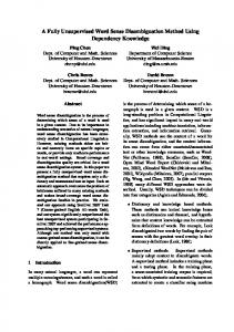
proves results. The same is observed for hypernym/hyponym gloss members. Using example sentence members of either synsets or their hypernymy/hyponymy synsets bring down the performance of the system. This is also justified when we consider only synset members, gloss members, hypernym/hyponym synset members, hypernym/hyponym gloss members which give a score close to the best obtained score. All the features (S, G, E, HS, HG & HE), when used together, give the best performance as shown in Table 5. Also, we have calculated the F-1 score for Hindi and English WSD for increasing thresholds on the frequency of nouns appearing in the corpus. This is depicted in Figure 2 and Figure 3 for Hindi and English WSD respectively. Here, in both plots, it is clearly shown that, as the frequency of nouns in the corpus increases our approach outperforms baselines for both Hindi and English WSD. On the other hand, SemCor baseline accuracy decreases for those words which occur more than 8 times in the test corpus. This is depicted in Figure 3. There are 15 such frequent word types. The main reason for low SemCor accuracy is that these words occur very few times with their MFS as listed by the SemCor baseline. For example, the word cell never appears with its MFS (as listed by SemCor baseline) in the SENSEVAL-2 dataset. As opposed to baselines, our approach gives a feasible way to extract predominant senses in an unsupervised setup. Our approach is domain independent sothat it can be very easily adapted to a domain specific corpus. To get the domain specific word embeddings, we simply have to run the word2vec program on the domain specific corpus. The domain specific word embeddings can be used to get the MFS for the domain of interest. Our approach is language independent. However, due to time and space constraints we have performed our experiments on only Hindi and English languages.

5

Related Work

McCarthy et al. (2007) proposed an unsupervised approach for finding the predominant sense using an automatic thesaurus. They used WordNet similarity for identifying the predominant sense. Their approach outperforms the SemCor baseline for words

Figure 2: UMFS-WE accuracy on Hindi WSD for words with various frequency thresholds in Newspaper dataset

with SemCor frequency below five. Buitelaar et al. (2001) presented the knowledge based approach for ranking GermaNet synsets on specific domains. Lapata et al. (2004) worked on detecting the predominant sense of verbs where verb senses are taken from the Levin classes. Our approach is similar to that of McCarthy et al. (2007) as we are also learning predominant senses from the untagged text.

6

Conclusion and Future Work

In our paper, we presented an unsupervised approach for finding the most frequent sense for nouns by exploiting word embeddings. Our approach is tested on Hindi and English WSD. It is found that our approach outperforms the WFS baseline for Hindi. As the frequency of noun increases in the corpus, our approach outperforms the baseline for both Hindi and English WSD. Our approach can be easily ported to various domains and across languages. In future, we plan to improve on the performance of our model for English, even for infrequent words. Also, we will explore this approach for other languages and for other parts-of-speech.

7

Acknowledgments

We would like to thank Mrs. Rajita Shukla, Mrs. Jaya Saraswati and Mrs. Laxmi Kashyap for their enormous efforts in the creation of the WordNet First Baseline for the Hindi WordNet. We also thank

Figure 3: UMFS-WE accuracy on English WSD for words with various frequency thresholds in SENSEVAL2 dataset

TDIL, DeitY for their continued support.

References Satanjeev Banerjee and Ted Pedersen. 2003. Extended Gloss Overlaps as a Measure of Semantic Relatedness. In Proceedings of the Eighteenth International Joint Conference on Artificial Intelligence, pp 805-810. Mohit Bansal, Kevin Gimpel and Karen Livescu. 2014. Tailoring Continuous Word Representations for Dependency Parsing. Proceedings of ACL 2014. Ondˇrej Bojar, Diatka Vojtˇech, Rychl´y Pavel, Straˇna´ k Pavel, Suchomel V´ıt, Tamchyna Aleˇs and Zeman Daniel. 2014. HindEnCorp - Hindi-English and Hindi-only Corpus for Machine Translation. Proceedings of the Ninth International Conference on Language Resources and Evaluation (LREC’14). Paul Buitelaar and Bogdan Sacaleanu. 2001. Ranking and selecting synsets by domain relevance. Proceedings of WordNet and Other Lexical Resources, NAACL 2001 Workshop. Xinxiong Chen, Zhiyuan Liu and Maosong Sun. 2014. A Unified Model for Word Sense Representation and Disambiguation. Proceedings of ACL 2014. Ronan Collobert, Jason Weston, L´eon Bottou, Michael Karlen, Koray Kavukcuoglu, Pavel P. Kuksa. 2011. Natural Language Processing (almost) from Scratch. CoRR, http://arxiv.org/abs/1103.0398. Agirre Eneko and Edmonds Philip. 2007. Word Sense Disambiguation: Algorithms and Applications. Springer Publishing Company, Incorporated, ISBN:1402068700 9781402068706.

Z. Harris. 1954. Distributional structure. Word 10(23):146-162. Tomas Mikolov, Chen Kai, Corrado Greg and Dean Jeffrey. 2013. Efficient Estimation of Word Representations in Vector Space. In Proceedings of Workshop at ICLR, 2013. Diana McCarthy, Rob Koeling, Julie Weeds and John Carroll. 2007. Unsupervised Acquisition of Predominant Word Senses. Computational Linguistics, 33 (4) pp 553-590. Mirella Lapata and Chris Brew. 2004. Verb class disambiguation using informative priors. Computational Linguistics, 30(1):45-75. Bengio Yoshua, Ducharme R´ejean, Vincent Pascal and Janvin Christian. 2003. A Neural Probabilistic Language Model. J. Mach. Learn. Res., issn = 1532-4435, pp 1137-1155.