tificially corrupted and real images and the performance is very close, and in some cases even ... Finally, if we substitute a Gaussian window to the hard disk-shaped window around the current ... In order to recover u : Rd â R from noisy ...
Unsupervised Patch-Based Image Regularization and Representation Charles Kervrann1,2 and J´erˆome Boulanger1,2 1
IRISA/INRIA Rennes, Projet Vista, Campus Universitaire de Beaulieu, 35 042 Rennes Cedex, France 2 INRA - MIA, Domaine de Vilvert, 78 352 Jouy-en-Josas, France
Abstract. A novel adaptive and patch-based approach is proposed for image regularization and representation. The method is unsupervised and based on a pointwise selection of small image patches of fixed size in the variable neighborhood of each pixel. The main idea is to associate with each pixel the weighted sum of data points within an adaptive neighborhood and to use image patches to take into account complex spatial interactions in images. In this paper, we consider the problem of the adaptive neighborhood selection in a manner that it balances the accuracy of the estimator and the stochastic error, at each spatial position. Moreover, we propose a practical algorithm with no hidden parameter for image regularization that uses no library of image patches and no training algorithm. The method is applied to both artificially corrupted and real images and the performance is very close, and in some cases even surpasses, to that of the best published denoising methods.
1
Introduction
Most of the more efficient regularization methods are based on energy functionals minimization since they are designed to explicitly account for the image geometry, involving the adjustment of global weights that balance the contribution of prior smoothness terms and a fidelity term [23, 28]. Thus, related partial differential equations (PDE) and variational methods have shown impressive results to tackle the problem of edge-preserving smoothing [24, 28, 32] and more recently the problem of image decomposition [1]. Moreover, other smoothing algorithms aggregate information over a neighborhood of fixed size, based on two basic criteria: a spatial criterion to select points in the vicinity of the current point and a brightness criterion in order to choose only points which are similar in some sense. In view of this generic approach, a typical filter is the sigma filter [19] and a continuous version of this filter gives the well-known nonlinear Gaussian filter [14]. Finally, if we substitute a Gaussian window to the hard disk-shaped window around the current position, we get variants of the bilateral filtering [31], controlled by setting the standard deviations in both spatial and brightness domains. Nevertheless, as effective as bilateral filtering and variants, they lacked a theoretical basis and some connections to better understood methods have been A. Leonardis, H. Bischof, and A. Prinz (Eds.): ECCV 2006, Part IV, LNCS 3954, pp. 555–567, 2006. c Springer-Verlag Berlin Heidelberg 2006 �
556
C. Kervrann and J. Boulanger
investigated. In particular, the relationships between bilateral filtering and iterative mean-shift algorithm, local mode filtering, clustering, local M-estimators, non-linear diffusion, regularization approaches combining nonlocal data and nonlocal smoothness terms, and Beltrami flow, can be found in [33, 11, 3, 22, 29]. Nevertheless, we note that all cited methods have a relatively small number of regularity parameters that control the global amount of smoothing being performed. They are usually chosen to give a good and global visual impression and are sometimes heuristically chosen [31]. Furthermore, when local characteristics of the data differ significantly across the image domain, selecting local smoothing parameters seems more satisfying and, for instance, has been addressed in [4, 13, 5, 8]. But, what makes image regularization very hard, is that natural images often contain many irrelevant objects. To develop better image enhancement algorithms that can deal with such a structured noise, we need explicit models for the many regularities and geometries seen in local patterns. This corresponds to another line of work which consists in modeling non-local pairwise interactions from training data [35] or a library of natural image patches [12, 27]. The idea is to improve the traditional Markov random field (MRF) models by learning potential functions from examples and extended neighborhoods for computer vision applications [35, 12, 27]. In our framework, we will also assume that small image patches in the semi-local neighborhood of a point contains the essential process required for local smoothing. Thus, the proposed patch-based regularization approach is conceptually very simple being based on the key idea of iteratively increasing a window at each pixel and adaptively weighting input data. The data points with a similar patch to the central patch will have larger weights in the average. We use 7 × 7 or 9 × 9 image patches to compute these weights since they are able to capture most of local geometric patterns and texels seen in images. Note also that, it has been experimentally confirmed that intuitive exemplar-based approaches are fearsome for 2D texture synthesis [10] and image inpainting [34, 9]. Nevertheless, we propose here a theoretical framework for choosing a semi-local neighborhood adapted to each pixel. This neighborhood which could be large, is chosen to balance the accuracy of the pointwise estimator and the stochastic error, at each spatial position [20]. This adaptation method is a kind of change-point detection procedure, initiated by Lepskii [20]. By introducing spatial adaptivity, we extend the work earlier described in [7] which can be considered as an extension of bilateral filtering [31] to image patches. The related works to our approach are the unsupervised recent non-local means algorithm [7], nonlinear Gaussian filters [31, 33, 22] and statistical smoothing schemes [25, 16, 17], but are enhanced via incorporating either a variable window scheme or patch-based weights. Finally, to our knowledge, the more related competitive methods for image denoising, are recent wavelet-based methods [30, 26]. In our experiments, we have then reported the results when these methods are applied to a commonly-used image dataset [26]. We show that the performance of our method surpasses most of the already published and very competitive denoising methods [30, 26, 27, 7].
Unsupervised Patch-Based Image Regularization and Representation
2
557
Patch-Based Approach
Consider the following basic image model: Yi = u(xi ) + εi , i = 1, . . . , |G| where xi ∈ G ⊂ Rd , d ≥ 2, represents the spatial coordinates of the discrete image domain of |G| pixels, and Yi ∈ R+ is the observed intensity at location xi . We suppose the errors εi to be independent, distributed Gaussian zero-mean random variables with unknown variances σ 2 . In order to recover u : Rd → R from noisy observations, we suppose there exists repetitive patterns in the semilocal neighborhood of a point xi . In particular, we assume that the unknown image u(xi ) can be calculated as the weighted average of input data over a variable neighborhood ∆i around that pixel xi . Henceforth, the points xj ∈ ∆i with a similar regularized patch uj to the reference regularized image patch ui will have larger weights in the average. Now, we just point out that our ambition is not to learn generic image priors from a database of image patches as already described in [35, 12, 27], but we just consider image patches as non-local image features, and adapt kernel regression techniques for image regularization. For simplicity, an image patch ui is modeled as a fixed size square window of p × p pixels centered at xi . In what follows, ui will denote indifferently a patch or a vector of p2 elements where the pixels are concatenated along a fixed lexicographic ordering. As with all exemplar-based techniques, the size of image patches must be specified in advance [10, 34, 9, 7]. We shall see that a 7×7 or 9×9 patch is able to take care of the local geometries and texture in the image while removing undesirable distortions. In addition, the proposed approach requires no training step and may be then considered as unsupervised. This makes the method somewhat more attractive for many applications. Another important question under such an estimation approach is how to determine the size and shape of the variable neighborhood (or window) ∆i at each pixel, from image data. The selected window must be different at each pixel to take into account the inhomogeneous smoothness of the image. For the sake of parsimony, the set N∆ of admissible neighborhoods will be arbitrarily chosen as a geometric grid of nested square windows N∆ = {∆i,n : |∆i,n | = (2n +1)×(2n +1), n = 1, . . . , N∆ }, where |∆i,n | = #{xj ∈ ∆i,n } is the cardinality of ∆i,n and N∆ is the number of elements of N∆ . For technical reasons, we will require the following conditions: ∆i,n is centered at xi and ∆i,n ⊂ ∆i,n+1 . Finally, we focus on the local L2 risk as an objective criterion to guide the optimal selection of the smoothing window for constructing the “best” possible estimator. This optimization will be mainly accomplished by starting, at each pixel, with a small window ∆i,0 as a pilot estimate, and increasing ∆i,n with n. The use of variable and overlapping windows combined with adaptive weights contributes to the regularization performance with no block effect. Adaptive estimation procedure. The proposed procedure is iterative [25, 17] and works as follows. At the initialization, we choose a local window ∆i,0 containing only the point of estimation xi (|∆i,0 | = 1). A first estimate u �i,0 (and 2 2 its variance υ�i,0 = Var(� ui,0 )) is then given by: u �i,0 = Yi and υ �i,0 = σ �2 where an estimated variance σ �2 has been plugged in place of σ 2 since the variance
558
C. Kervrann and J. Boulanger
of errors are supposed to be unknown. At the next iteration, a larger window ∆i,1 with ∆i,0 ⊂ ∆i,1 centered at xi is considered. Every point xj from ∆i,1 gets a weight πi∼j,1 defined by comparing pairs of p × p regularized patches �T �T � � (1) (p2 ) (1) (p2 ) � i,0 = u � j,0 = u u �i,0 , · · · , u �i,0 and u �j,0 , · · · , u �j,0 obtained at the first iteration. Note that p is fixed for all the pixels in the image. As usual, the points xj � i,0 will have weights close to 1 and 0 otherwise. Then we with a similar patch to u recalculate an new estimate u �i,1 defined as the weighted average of data points lying in the neighborhood ∆i,1 . We continue this way, increasing with n the considered window ∆i,n while n ≤ N∆ where N∆ denotes the maximal number of iterations of the algorithm. For each n ≥ 1, the studied maximum likelihood 2 �i,n can be then represented as (ML) estimator u �i,n and its variance υ � � 2 2 u �i,n = πi∼j,n Yj , υ �i,n = σ �2 [πi∼j,n ] (1) xj ∈∆i,n
xj ∈∆i,n
where the weights πi∼j,n � are continuous variables and satisfy the usual conditions 0 ≤ πi∼j,n ≤ 1 and xj ∈∆i,n πi∼j,n = 1. In our modeling, these weights are � i,n−1 and u � j,n−1 obtained at computed from pairs of regularized p × p patches u iteration n − 1 and p is fixed for all the pixels in the image. In what follows, n will coincide with the iteration and we will use n �(xi ) to designate the index of def def � i) = ∆ �i,�n(x ) and the “best” estimate u the “best” window ∆(x �(xi ) = u �i,�n(xi ) . i Among all non-rejected window ∆i,n from N∆ , the optimal window is chosen as � i ) = arg max {|∆i,n | : |� ∆(x ui,n − u �i,n� | ≤ � υ �i,n� , for all 1 ≤ n� < n} ∆i,n ∈N∆
where � is a positive constant. Throughout this paper, we shall see the rational behind this pointwise statistical rule and the proposed strategy that updates the pointwise estimator when the neighborhood increases at each iteration [25]. � i,n Adaptive weights. In order to compute the similarity of between patches u � j,n , a distance must be first considered. In [10, 34, 9, 7], several authors and u � j,n �2 is a reliable measure to compare showed that the L2 distance �� ui,n − u image patches. To make a decision, we have rather used a normalized distance 1 � � −1 (� � j,n−1 ) = � j,n−1 )T V � j,n−1 ) (2) dist(� ui,n−1 , u (� ui,n−1 − u i,n−1 ui,n−1 − u 2 � � −1 (� � i,n−1 )T V � i,n−1 ) + (� uj,n−1 − u j,n−1 uj,n−1 − u � ·,n−1 is p2 × p2 diagonal matrix of the form (the symbol “·” is used to where V denote a spatial position) �2 ⎞ ⎛� (1) 0 ··· 0 υ �·,n−1 ⎟ ⎜ ⎟ .. .. .. .. � ·,n−1 = ⎜ V ⎟ ⎜ . . . . ⎝ � 2 �2 ⎠ (p ) 0 ··· 0 υ �·,n−1
Unsupervised Patch-Based Image Regularization and Representation (�)
559 (�)
and υ �·,n−1 , � = 1, · · · , p2 , is the local standard deviation of the estimator u �·,n−1 , � ·,n−1 = and the index � is used to denote a spatial position in an image patch u � �T (1) (�) (p2 ) u �·,n−1 , · · · , u �·,n−1 , · · · , u �·,n−1 . Moreover, we used a symmetrized distance to test both the hypotheses that xj belongs to the region ∆i,n and xi belongs to the � i,n−1 and u � j,n−1 are region ∆j,n , at the same time. Accordingly, the hypothesis u � j,n−1 ) ≤ λα . In our similar, is accepted if the distance is small, i.e. dist(� ui,n−1 , u modeling, the parameter λα ∈ R+ is chosen as a quantile of a χ2p2 ,1−α distribution with p2 degrees of freedom, and controls the probability of type I error for the � j,n−1 ) ≤ hypothesis of two points to belong to the same region: P {dist(� ui,n−1 , u λα } = 1 − α. All these tests (|∆i,n | tests) have to be performed at a very high significance level, our experience suggesting to use a 1 − α = 0.99-quantile. Henceforth, we introduce the following commonly-used weight function � � � j,n−1 ) K λ−1 ui,n−1 , u α dist(� � πi∼j,n = (3) � � � j,n−1 ) K λ−1 ui,n−1 , u α dist(� xj ∈∆i,n
with K(·) denoting a monotone decreasing function, e.g. a kernel K(x) = exp(−x/2). Due to the fast decay of the exponential kernel, large distances between estimated patches lead to nearly zero weights. Note that the use of weights enables to relax the structural assumption the neighborhood is a variable square window. An “ideal” smoothing window. In this section, we address the problem of the automatic selection of the window ∆i,· adapted for each pixel xi . It is well understood that the local smoothness varies significantly for point to point in the image and global risk measures cannot wholly reflect the performance of estimators at a point. Then, a classical way to measure the performance of the estimator u �i,n to its target value u(xi ) is to choose the local L2 risk, which is 2 �i,n : explicitly decomposed into the sum of the squared bias �b2i,n and variance υ � �1/2 2 1/2 E|� ui,n − u(xi )|2 = |�b2i,n + υ �i,n | .
(4)
Our goal is then to minimize this local L2 risk with respect to the size of the window ∆i,n , at each pixel in the image. Actually, the optimal solution explicitly depends on the smoothness of the “true” function u(xi ) which is unknown, and so, of less practical interest [16]. A natural way to bring some further understanding of the situation is then to individually analyze the behavior of the bias and variance terms when ∆i,n increases or decreases with n as follows: ui,n − u(xi )] is nonrandom and characterizes the – The bias term �bi,n = E [� accuracy of approximation of the function u at the point xi . As it explicitly depends on the unknown function u(xi ), its behavior is√ doubtful. Nevertheless, if we use the geometric inequality |xj − xi | ≤ 22 |∆i,n |1/2 and assume that there exists a real constant 0 < C1 < ∞ such that
560
C. Kervrann and J. Boulanger
C1 |u(xj ) − u(xi )| ≤ C1 |xj − xi |, then |�bi,n | ≤ √ |∆i,n |1/2 . Accordingly, |�bi,n |2 2 is of the order O(|∆i,n |) and typically increases when ∆i,n increases (see also [16]). – The behavior of the variance term is just opposite. The errors are indepen2 dent and the stochastic term υ �i,n can be �exactly computed on the basis of observations. Since 0 ≤ πi∼j,n ≤ 1 and xj ∈∆i,n πi∼j,n = 1, it follows that 2 ≤ σ �2 . In addition, we can reasonably assume that there σ �2 |∆i,n |−1 ≤ υ�i,n 2 2 2 ≈ σ �2 |∆i,n |−γ . Accordingly, as exits a constant 0 ≤ γ ≤ 1 such that υ�i,n 2 �i,n , and so υ �i,n ∆i,n increases, more data is used to construct the estimate u decreases.
Therefore, the bias and standard deviation terms are monotonous functions with opposite behaviors. In order to approximately minimize the local L2 risk with respect to |∆i,n |, a natural idea would be to minimize an upper bound of the form 2 C2 �2 |∆i,n |−γ . E|� ui,n − u(xi )|2 ≤ 1 |∆i,n | + σ 2 � � 1
Unfortunately, the size of the optimal window defined as |∆� (xi )| = 2γC 2σ� 1 cannot be used in practice since C1 and γ are unknown. However, for this optimal solution |∆� (xi )|, it can be easily shown that the ratio between the optimal bias b� (xi ) and the optimal standard deviation υ � (xi ) is not image dependent, i.e. |b� (xi )| ≤ γυ � (xi ). Accordingly, the ideal window will be chosen as the largest window ∆i,n such that �bi,n is still not larger than γ� υi,n , for some real value 0 ≤ γ 2 ≤ 1: ∆� (xi ) = sup∆i,n ∈N∆ {|∆i,n | : �bi,n ≤ γ� υi,n }. Now, we just point out that the estimator u �i,n is usually decomposed as 2 � u �i,n = u(xi ) + bi,n + νi where νi ∼ N (0, E[νi ]). Hence, E[� ui,n ] = u(xi ) + �bi,n , def 2 E[νi2 ] = E[|� ui,n − u(xi ) − �bi,n |2 ] = υ�i,n and the following inequality |� ui,n − u(xi )| ≤ �bi,n + κ υ �i,n holds with a high probability for 0 < κ < ∞. Accordingly, we can modify the previous definition of the ideal window as follows 2
∆� (xi ) =
sup {|∆i,n | : |� ui,n − u(xi )| ≤ (γ + κ) υ�i,n },
∆i,n ∈N∆
2
γ 2 +1
(5)
which depends no longer on �bi,n . In the next section, we shall see that a practical data-driven window selector based on this definition of ∆� (xi ) which is yet related to the ideal and unobserved function u(xi ), can actually be derived. A data-driven local window selector. In our approach, the collection of esti�(xi )} is naturally ordered in the direction of increasing |∆i,n | mators {� ui,1 , . . . , u where u �(xi ) can be thought as the best possible estimator with the smallest variance. A selection procedure can be then described based on pairwise comparisons of an essentially one-dimensional family of competing estimators u �i,n . In this modeling, the differences u �i,n − u �i,n� are Gaussian random variables with 2 � �i,n� ) ≤ υ �i,n known variances Var(� ui,n − u � with 1 ≤ n < n , and expectations equal to the bias differences �bi,n − �bi,n� . From the definition of ∆� (xi ) (see (5)),
Unsupervised Patch-Based Image Regularization and Representation
561
we derive |� ui,n� − u �i,n | ≤ (2γ + κ)� υi,n� , 1 ≤ n� < n, and, among all good candidates {� ui,n } satisfying this inequality, one choose the one with the smallest 2 variance υ �i,n . Following the above discussion, a window selector will be then based on the following pointwise rule [20, 21]: � i ) = arg max {|∆i,n | : |� ui,n − u �i,n� | ≤ � υ �i,n� , for all 1 ≤ n� < n} (6) ∆(x ∆i,n ∈N∆
where � = (2γ+κ). This rule actually ensures the balance between the stochastic term and the bias term, and means that we take the largest window such that the estimators u �i,n and u �i,n� are not too different, in some sense, for all 1 ≤ n� < n (see [18]). Hence, if an estimated point u �i,n� appears far from the previous ones, this means that the bias is already too large and the window ∆i,n is not a good one. This idea underlying our construction definitely belongs to Lepskii [20, 21]. Implementation. At the initialization, we naturally choose |∆i,0 | = 1, the fixed size of p × p patches and choose the number of iterations N∆ . In addition, the noise variance σ �2 is robustly estimated from input data (see [17]). To complete
Algorithm.
Let {p, α, �, N∆ } be the parameters
2 Initialization: compute σ � 2 and set u �i,0 = Yi and υ �i,0 =σ � 2 for each xi ∈ G.
Repeat – for each xi ∈ G • compute
� � � j,n−1 ) K λ−1 ui,n−1 , u α dist(� � � −1 � � j,n−1 ) K λα dist(� ui,n−1 , u
πi∼j,n =
xj ∈∆i,n
�
u �i,n =
xj ∈∆i,n
πi∼j,n Yj ,
2 υ �i,n =σ �2
�
[πi∼j,n ]2
xj ∈∆i,n
• choose the window as � i ) = arg ∆(x
max
∆i,n ∈N∆
�
� ui,n − u �i,n� | ≤ � υ �i,n� , for all 1 ≤ n� < n . |∆i,n | : |�
If this rule is violated at iteration n, we do not accept u �i,n and keep the estimate �(xi ) = u �i,n−1 and n � (xi ) = n − 1. This u �i,n−1 as the final estimate at xi , i.e. u estimate is unchanged at the next iterations and xi is “frozen”. – increment n while n ≤ N∆ .
Fig. 1. Patch-based image regularization algorithm
562
C. Kervrann and J. Boulanger
the procedure, we choose � ∈ [2, 4] in order to get a good accuracy for the pointwise estimator (see [18] for the proof) and λα as a 1 − α = 0.99-quantile of a χ2p2 ,1−α distribution. Finally, the complexity of the algorithm given in Fig. 1, is of the order p × p × |G| × (|∆·,1 | + . . . + |∆·,N∆ |).
3
Experimental Results
Our results were measured by the peak signal-to-noise � ratio (psnr) in decibels (db) as psnr = 10 log10 (2552 /MSE) with MSE = |G|−1 xi ∈G (uo (xi ) − u �(xi ))2 where u0 is the noise-free original image. We have done simulations on a commonlyused set of images available at http://decsai.ugr.es/∼javier/denoise/test images/ and described in [26]. In all our experiments, we have chosen image patches of 9 × 9 pixels and set the algorithm parameters as follows: λ0.01 = χ281,0.01 = 113.5, � = 3 and N∆ = 4 (see [18]). The processing of a 256 × 256 image required typically about 1 minute (p = 9) on a PC (2.0 Ghz, Pentium IV) using a C++ implementation. The potential of the estimation method is mainly illustrated with the 512 × 512 lena image (Fig. 2a) corrupted by an additive white-Gaussian noise (WGN) (Fig. 2b, psnr = 22.13 db, σ = 20). In Fig. 2c, the noise is reduced in a natural manner and significant geometric features, fine textures, and original contrasts are visually well recovered with no undesirable
Fig. 2. Denoising of the artificially corrupted lena image (WGN, σ = 20)
Unsupervised Patch-Based Image Regularization and Representation
563
Fig. 3. Denoising results on the noisy lena image (WGN, σ = 20). a) Our method (psnr = 32.64), b) NL-means filter [7] (psnr=31.09), c) Fields-of-Experts [27] (psnr=31.92), d) wavelet-based denoising method (BLS-GSM) [26] (psnr=32.66).
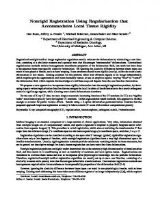
Fig. 4. Detail of the barbara image. From left to right: original image, artificially corrupted image (WGN, σ = 30), result of our patch-based method, difference between the noisy image and the regularized image (noise component).
artifacts (psnr = 32.64 db). The noise component is shown in Fig. 2e (magnification factor of 2) and has been estimated by calculating the difference between the noisy image (Fig. 2b) and the recovered image (Fig. 2c). The estimated noise component contains few geometric structures and is similar to a simulated white Gaussian noise. To better appreciate the accuracy of the denoising pro�(xi ) is shown in Fig. 2d cess, the variance υ �2 (xi ) of the pointwise estimator u where dark values correspond to high-confidence estimates. As expected, pixels with a low level of confidence are located in the neighborhood of image discon� i ): � (xi ) occurring in ∆(x tinuities. Figure 2f shows the probability of a patch u def � i )} = #Ω(xi )/|∆(x � i )| where Ω(xi ) is used to denote P{� u(xi ) occurring in ∆(x � � (xj )) ≤ λα }. In Fig. 2f, dark values correspond the set {xj ∈ ∆(xi ) : dist(� u(xi ), u low probabilities of occurrence and, it is confirmed that repetitive patterns in the neighborhood of image discontinuities are mainly located along image edges. Our approach is also compared to the non-local means algorithm [7] using 7 × 7 image patches and a fixed search window of 21 × 21 pixels as recommended by the authors: the visual impression and the numerical results are improved using our algorithm (see Fig. 3b). Finally, we have compared the performance of our method to the Wiener filtering (WF) (Matlab function wiener2) and other competitive methods [28, 31, 24], including recent patch-based approaches [7, 27] and pointwise adaptive estimation approaches [25, 17]. We point out that, visually
564
C. Kervrann and J. Boulanger
Fig. 5. Real noisy photographs (top) and restoration results (bottom)
noisy (left) and denoised (middle) y − t images, and variance image (right)
noisy (top) and denoised (middle) x − t images, and variance image (bottom)
Fig. 6. Results on a 2D image depicting trajectories of vesicles of transport in the spatio-temporal planes y − t (left) and x − t (right) (analysis of Rab proteins involved in the regulation of transport from the Golgi apparatus to the endoplasmic reticulum).
and quantitatively, our very simple and unsupervised algorithm favorably compares to any of these denoising algorithms, including the more sophisticated and best known wavelet-based denoising methods [30, 26] (see Fig. 3d) and learned filters-based denoising methods [27] (see Fig. 3c). In Table 1 (a), we reported the best available published psnr results for the same image dataset [26] ; we note that our method nearly outperforms any of the tested methods in terms of psnr. Also, if the psnr gains are marginal for some images, the visual difference can be significant as shown in Fig. 3 where less artifacts are visible using our method (see also Fig. 4). Nevertheless, other competitive unsupervised patchbased methods exist (e.g. see [15, 2]), but we did not report the results on this
Unsupervised Patch-Based Image Regularization and Representation
565
Table 1. Performances of our method when applied to test noisy (WGN) images Image σ/psnr Our method Buades et al. [7] Kervrann [17] Polzehl et al. [25] Portilla et al. [26] Roth et al. [27] Rudin et al. [28] Starck et al. [30] Tomasi et al. [31] Wiener filering
Lena 20/22.13
Barbara 20/22.18
Boats 20/22.17
House 20/22.11
Peppers 20/22.19
32.64 31.09 30.54 29.74 32.66 31.92 30.48 31.95 30.26 28.51
30.37 29.38 26.50 26.05 30.32 28.32 27.07 27.02 26.99
30.12 28.60 28.01 27.74 30.38 29.85 29.02 28.41 27.97
32.90 31.54 30.70 30.31 32.39 32.17 31.03 30.01 28.74
30.59 29.05 28.23 28.40 30.31 30.58 28.51 28.88 28.10
(a) Performances of denoising algorithms when applied to test noisy (WGN) images. σ/psnr 5 / 34.15 10 / 28.13 15 / 24.61 20 / 22.11 25 / 2017 50 / 14.15 75 / 10.63 100 / 8.13
Lena Barbara Boats 5122 5122 5122 37.91 37.12 36.14 35.18 33.79 33.09 33.70 31.80 31.44 32.64 30.37 30.12 31.73 29.24 29.20 28.38 24.09 25.93 25.51 22.10 23.69 23.32 20.64 21.78
House Peppers 2562 2562 37.62 37.34 35.26 34.07 34.08 32.13 32.90 30.59 32.22 29.73 28.67 25.29 25.49 22.31 23.08 20.51
(b) Performances of our method (p = 9, N∆ = 4, α = 0.01) for different signal-to-noise ratios (WGN).
patch Lena Barbara Boats House Peppers size 5122 5122 5122 2562 2562 3 × 3 32.13 28.97 29.86 32.69 30.86 5 × 5 32.52 29.97 30.15 33.05 30.98 7 × 7 32.63
30.27
30.17
33.03
30.80
9 × 9 32.64
30.37
30.12
32.90
30.59
(c) Performances of our method (N∆ = 4, α = 0.01) for different patch sizes (WGN, σ = 20)
image dataset since they are not available. These methods must be considered for future comparisons. To complete the experiments, Table 1 (b) shows the psnr values using our patch-based regularization method when applied to this set of test images for a wide range of noise variance. Moreover, we have also examined some complementary aspects of our approach. Table 1 (c) shows the psnr values obtained by varying the patch size. Note the psnr values are close for every patch size and the optimal patch size depends on the image contents. Nevertheless, a patch 9 × 9 seems appropriate in most cases and a smaller patch can be considered for processing piecewise smooth images. In the second part of experiments, the effects of the patch-based regularization is approach are illustrated on real old photographs. The set of parameters is unchanged for processing all these test images: p = 9, N∆ = 4, α = 0.01. In most cases, a good compromise between the amount of smoothing and preservation of edges and textures is automatically reached. In that case, the noise variance σ �2 is automatically estimated from image data. The reconstruction of images is respectively shown in Fig. 5. Note that geometric structures are well preserved and the noise component corresponding to homogeneous artifacts is removed. Finally, we have applied the patch-based restoration method to noisy 2D images extracted from a temporal 2D+time (xy − t) sequence of 120 microscopy images in intracellular biology, showing a large number of small fluorescently labeled moving vesicles in regions close to the Golgi apparatus (courtesy of Curie Institute). The reading of observed trajectories is easier if the patch-based
566
C. Kervrann and J. Boulanger
estimation method is applied to both noisy x−t or y −t projection images shown in Fig. 6 (see also [6]).
4
Conclusion
We have described a novel adaptive regularization algorithm where patch-based weights and variable window sizes are jointly used. The use of variable and overlapping windows contributes to the regularization performance with no block effect, enhances the flexibility of the resulting local regularizers and make them possible to cope well with spatial inhomogeneities in natural images. An advantage of the method is that internal parameters can be easily chosen and are relatively stable. The algorithm is able to regularize both piecewise-smooth and textured natural images since they contain enough redundancy. Actually, the performance of our simple algorithm is very close to that of the best already published denoising methods. In the future, we plan to study the automatic patch size selection to better adapt to image contents.
References 1. Aujol, J.F., Aubert, G., Blanc-Fraud, L., Chambolle, A.: Image decomposition into a bounded variation component and an oscillating component. J. Math. Imag. Vis. 22 (2005) 71-88 2. Awate, S.P., Whitaker, R.T.: Higher-order image statistics for unsupervised, information-theoretic, adaptive, image filtering. In: Proc. CVPR’05, San Diego (2005) 3. Barash, D., Comaniciu, D.: A Common framework for nonlinear diffusion, adaptive smoothing, bilateral filtering and mean shift. Image Vis. Comp. 22 (2004) 73-81 4. Black, M.J., Sapiro, G.: Edges as outliers: anisotropic smoothing using local image statistics. In: Proc. Scale-Space’99, Kerkyra (1999) 5. Brox, T., Weickert, J.: A TV flow based local scale measure for texture discrimination. In: Proc. ECCV’04, Prague (2004) 6. Boulanger, J., Kervrann, C., Bouthemy, P.: Adaptive spatio-temporal restoration for 4D fluoresence microscopic imaging. In: Proc. MICCAI’05, Palm Springs (2005) 7. Buades, A., Coll, B., Morel, J.M.: Image denoising by non-local averaging. In: Proc. CVPR’05, San Diego (2005) 8. Comaniciu, D., Ramesh, V., Meer, P.: The variable bandwidth mean-shift and data-driven scale selection. In: Proc. ICCV’01, Vancouver (2001) 9. Criminisi, A., P´erez, P., Toyama, K.: Region filling and object removal by exemplarbased inpainting. IEEE T. Image Process. 13 (2004) 1200-1212 10. Efros, A., Leung, T.: Texture synthesis by non-parametric sampling. In: Proc. ICCV’99, Kerkyra (1999) 11. Elad, M.: On the bilateral filter and ways to improve it. IEEE T. Image Process. 11 (2002) 1141-1151 12. Freeman, W.T., Pasztor, E.C., Carmichael, O.T.: Learning low-level vision. Int. J. Comp. Vis. 40 (2000) 25-47 13. Gilboa, G., Sochen, N., Zeevi, Y.Y.: Texture preserving variational denoising using an adaptive fidelity term. In: Proc. VLSM’03, Nice (2003)
Unsupervised Patch-Based Image Regularization and Representation
567
14. Godtliebsen, F., Spjotvoll, E., Marron, J.S.: A nonlinear Gaussian filter applied to images with discontinuities. J. Nonparametric Stat. 8 (1997) 21-43 15. Jojic, N., Frey, B., Kannan, A.: Epitomic analysis of appearance and shape. In: Proc. ICCV’03, Nice (2003) 16. Katkovnik, V., Egiazarian, K., Astola, J.: Adaptive window size image denoising based on intersection of confidence intervals (ICI) rule. J. Math. Imag. Vis. 16 (2002) 223-235 17. Kervrann, C.: An adaptive window approach for image smoothing and structures preserving. In: Proc. ECCV’04, Prague (2004) 18. Kervrann, C., Boulanger, J.: Local adaptivity to variable smoothness for exemplarbased image denoising and representation. INRIA RR-5624 (2005) 19. Lee, J.S.: Digital image smoothing and the sigma filter. Comp. Vis. Graph. Image Process. 24 (1983) 255-269 20. Lepskii, O.: On a problem of adaptive estimation on white Gaussian noise. Th. Prob. Appl. 35 (1980) 454-466 21. Lepskii, O.V., Mammen, E., Spokoiny, V.G.: Optimal spatial adaptation to inhomogeneous smoothness: an approach based on kernel estimates with variable bandwidth selectors. Ann. Stat. 25 (1997) 929-947 22. Mrazek, P., Weickert, J., Bruhn, A.: On robust estimation and smoothing with spatial and tonal kernels. Preprint 51, U. Bremen (2004) 23. Mumford, D., Shah, J.: Optimal approximations by piecewise smooth functions and variational problems. Comm. Pure and Appl. Math. 42 (1989) 577-685 24. Perona. P., Malik, J.: Scale space and edge detection using anisotropic diffusion. IEEE T. Patt. Anal. Mach. Intell. 12 (1990) 629-239 25. Polzehl, J., Spokoiny, V.: Adaptive weights smoothing with application to image restoration. J. Roy. Stat. Soc. B 62 (2000) 335-354 26. Portilla, J., Strela, V., Wainwright, M., Simoncelli, E.: Image denoising using scale mixtures of Gaussians in the wavelet domain. IEEE T. Image Process. 12 (2003) 1338-1351 27. Roth, S., Black, M.J.: Fields of experts: a framework for learning image priors with applications. In: Proc. CVPR’05, San Diego (2005) 28. Rudin, L., Osher, S., Fatemi, E.: Nonlinear Total Variation based noise removal algorithms. Physica D (2992) 60 (1992) 259-268 29. Sochen, N., Kimmel, R., Bruckstein, A.M.: Diffusions and confusions in signal and image processing. J. Math. Imag. Vis. 14 (2001) 237-244 30. Starck, J.L., Candes, E., Donoho, D.L.: The Curvelet transform for image denoising. IEEE T. Image Process. 11 (2002) 670-684 31. Tomasi, C., Manduchi, R.: Bilateral filtering for gray and color images. In: Proc. ICCV’98, Bombay (1998) 32. Tschumperl´e, D.: Curvature-preserving regularization of multi-valued images using PDE’s. In: Proc. ECCV’06, Graz (2006) 33. van de Weijer, J., van den Boomgaard, R.: Local mode filtering. In: Proc. CVPR’01, Kauai (2001) 34. Zhang, D., Wang, Z.: Image information restoration based on long-range correlation. IEEE T. Circ. Syst. Video Technol. 12 (2002) 331-341 35. Zhu, S.C., Wu, Y., Mumford, D.: Filters, random fields and maximum entropy (FRAME): Towards a unified theory for texture modeling. Int. J. Comp. Vis. 27 (1998) 107-126