Unsupervised Image-Set Clustering Using an Information Theoretic Framework Jacob Goldberger University of Toronto,
[email protected]
Shiri Gordon, Hayit Greenspan Tel-Aviv University, Tel-Aviv 69978, Israel Abstract
In this paper we combine discrete and continuous image models with informationtheoretic based criteria for unsupervised hierarchical image-set clustering. The continuous image modeling is based on mixture of Gaussian densities. The unsupervised image-set clustering is based on a generalized version of a recently introduced information-theoretic principle, the information bottleneck (IB) principle. Images are clustered such that the mutual information between the clusters and the image content is maximally preserved. Experimental results demonstrate the performance of the proposed framework for image clustering on a large image-set. Information theoretic tools are used to evaluate cluster quality. Particular emphasis is placed on the application of the clustering for efficient image search and retrieval.
Keywords: image clustering, mixture of Gaussians, mutual information, Kullback-Leibler divergence, information bottleneck, image database management, hierarchical database analysis, image modeling, retrieval.
Corresponding author: Dr. Hayit Greenspan Department of Biomedical Engineering Faculty of Engineering Tel Aviv University Tel Aviv 69978, Israel Phone: +972-3-6407398 Fax: +972-3-6407939 email :
[email protected]
1
Introduction
In recent years there has been a growing interest in developing effective methods for searching large image databases based on image content. Most approaches to image database management have focused on “search-by-query” (e.g., Flickner et al. [10], Ogle and Stonebraker [22], Pentland et al. [23], Smith and Chang [29], Carson et al. [4]). The users provide an example image for the query, following which the database is searched exhaustively for images that are most similar. The query image can be an existing image in the database or can be composed by the user. The similarity between the images in the database is determined by the selected feature-space representation (e.g., color, texture) and the distance measures used between the image representations. The color feature has been used as a test-bed for much algorithmic development in the field (such as the systems references above). Based on this representation space, the image content that we are focusing on is the image color content. Users often require a browsing mechanism (for example, to extract a good query image). A high quality browsing environment enables the users to find images by navigating through the database in a structured manner. For example hierarchically clustering the database into a tree structure, imposes a coarse to fine representation of image content within clusters and enables the users to navigate up and down the tree levels (e.g., Krishnamachari and AbdelMottaleb [19, 18], Chen et al. [6], Barnard et al. [1]). Multidimensional scaling (MDS) has been used as an alternative approach to database browsing by mapping images onto a two dimensional plane (Rubner et al. [24]). A key step for structuring a given database and for efficient search, is image content clustering. The goal is to find a mapping of the archive images into classes (clusters) such that the set of classes provides essentially the same prediction, or information, about the image archive as the entire image-set collection. The generated classes provide a concise summarization and visualization of the image content. The clustering process may be a supervised process using human intervention, or an unsupervised process. Hierarchical clustering procedures can be either agglomerative (start with each sample as a cluster and successively merge clusters, bottom-up) or divisive (start with all samples in one cluster and successively split clusters, top-down). Finally, the definition of a clustering scheme requires the determination 1
of two major components in the process: the input representation space (feature space used, global vs. local information) and the distance measure defined in the selected feature space. In works that use supervised clustering, the expert incorporates a-priori knowledge, such as the number of classes present in the database and representative icons for the different classes in the database. In Huang et al. [17], a hierarchical classification tree is generated via supervised learning, using a training set of images with known class labels. The tree is next used to categorize new images entered into the database. Sheikholeslami et al. [25] used a-priori defined image icons as cluster models (number of clusters given). Images are categorized in clusters on the basis of their similarity to the set of iconic images. The cluster icons are application dependent and are determined by the application expert. The clustering process is then performed in an unsupervised manner. Carson et al. [3] used a naive Bayes algorithm to learn image categories in a supervised learning scheme. The images are represented by a set of homogeneous regions in color and texture feature space, based on the “Blobworld” image representation (Carson et al. [4]). A probabilistic and continuous framework for supervised image category modeling and matching was introduced by Greenspan et al. [14]. Each image or image-set (category) is represented as a Gaussian mixture distribution (GMM). Images (categories) are compared and matched via a probabilistic measure of similarity between distributions known as the Kullback-Leibler (KL) distance. The GMMKL framework has been used recently in a variation of the K-means algorithm (top-down) for supervised and unsupervised clustering (Greenspan et al. [15]). The main drawback of supervised clustering is that it requires human intervention. In order to extract the cluster representation, the various methods require a-priori knowledge regarding the database content. This approach is therefore not appropriate for large unlabeled databases. A different set of studies is based on unsupervised clustering, where the clustering process is fully automated. Chen et al. [6] focus on the use of hierarchical tree-structures to both speed-up search-by-query (top-down) and organize databases for effective browsing (bottom-up). An hierarchical browsing environment (“similarity pyramid”) is constructed based on the results of the agglomerative clustering algorithm. The similarity pyramid groups similar images together, while allowing users to view the database at varying levels of detail. The image representation in that work combines global color, texture and edge histograms. The L1 norm is used as a distance measure between image representations 2
for the retrieval scheme. More localized representations are used by Abdel-Mottaleb et al. [18, 19]. They use local color histograms along with the histogram-intersection distance measure. Images in the database are divided into rectangular regions and represented by a set of normalized histograms corresponding to these regions. Each cluster centroid is computed as the average of the histograms in the corresponding image-set. An agglomerative clustering algorithm is used to create a tree structure which can serve as a browsing environment [19]. A statistical model for hierarchically structuring image collections is presented by Barnard et al. [1, 2]. The model integrates visual information within the image with semantic information provided by associated text. In this paper we propose a novel unsupervised image clustering algorithm utilizing the information bottleneck (IB) method. The IB principle is applied to both discrete and continuous image representations, using discrete image histograms and probabilistic continuous image modeling based on the Gaussian mixture distribution, respectively. The IB method was introduced by Tishby et al. [30] as a method for solving the problem of unsupervised data clustering and data classification. Thus far, this method has been demonstrated in the unsupervised classification of discrete objects sets given discrete features (e.g. documents [26, 28], galaxies [27], and image segmentation [16]). The case of compressing a Gaussian random variable given another correlated Gaussian r.v. was discussed in [5]. A version of the IB for clustering a discrete object set, given continuous features, is developed in detail in this paper (a short version was recently introduced by the authors [11], [13]). The rest of the paper is organized as follows. The continuous probabilistic image modeling scheme is presented in Section 2. Section 3 presents a derivation of the information bottleneck principle from the classical Shannon’s rate-distortion theory. In Section 4 we extend the information bottleneck principle to the case of continuous densities. An investigative analysis of the IB framework for clustering both discrete and continuous image representations, is presented in Section 5. Clustering quality is evaluated using both pre-labeled image-sets, as well as information-theoretic based measures. A discussion concludes the paper in Section 6.
3
Figure 1: Input image (left); Image modeling via Gaussian mixtures (right).
2
Image Modeling via Mixture of Gaussians
In this section we briefly review the concept of continuous image modeling using a mixture of Gaussians [4] [14]. We model an image as a set of coherent regions in feature space. We use the (L,a,b) color space. In order to include spatial information, the (x, y) position of the pixel is appended to the feature vector. The representation model is a general one and can incorporate other features (such as texture). Pixels are grouped into homogeneous regions which are represented by Gaussian distributions, and the entire image is thus represented by a Gaussian mixture model. The distribution of a d-dimensional random variable y is a mixture of k Gaussians if its density function is: f (y) =
k X i=1
αi q
1 exp{− (y − µi )T Σ−1 i (y − µi )}. 2 (2π)d |Σi | 1
(1)
The Expectation-Maximization (EM) algorithm [8] is used to determine the maximum likelihood parameters of the model. The Minimum Description Length (MDL) principle serves to select among values of k. In our experiments, k ranges from 3 to 8. A detailed review of various methods for estimating the number of the components appears in [9]. Figure 1 shows two examples of image modeling using Gaussian mixtures. In this visualization the Gaussian mixture is shown as a set of ellipsoids. Each ellipsoid represents the support, mean color and spatial layout, of a particular Gaussian in the image plane. In [14] the Kullback-Leibler (KL) divergence was proposed as a similarity measure between images. The KL-divergence is an information-theoretic measure for estimating the distances between discrete or continuous distributions (Kullback [20]). In case of a discrete (histogram) representation, the KL-measure can be easily obtained. However, there is no closed-form expression for the KL-divergence between two mixtures of Gaussians. We can use, instead, Monte-Carlo simulations to approximate the KL-divergence between distribu-
4
tions f and g: D(f ||g) =
Z
f log
n f f (xt ) 1X log ≈ g n t=1 g(xt )
such that x1 , ..., xn are sampled from f (x). Alternative deterministic approximations of the KL-divergence between Gaussian mixtures were suggested by Vasconcelos [32] and Goldberger et al. [12].
3
The Information Bottleneck Principle
The information bottleneck (IB) is an information theoretic principle recently introduced by Tishby, Pereira and Bialek [30]. The IB clustering method states that among all the possible clusterings of a given object set into a fixed number of clusters, the desired clustering is the one that minimizes the loss of mutual information between the objects and the features extracted from them. Assume there is a joint distribution p(x, y) on the “object” space X ˆ such that, and the “feature” space Y . According to the IB principle we seek a clustering X ˆ the information loss I(X; Y ) − I(X; ˆ Y) given a constraint on the clustering quality I(X; X), ˆ is the mutual information between X and X ˆ which is given by: is minimized. I(X; X) ˆ = I(X; X)
X
p(x)p(ˆ x|x) log
x,ˆ x
p(ˆ x|x) . p(ˆ x)
The IB principle can be motivated from Shannon’s rate-distortion theory (Cover and Thomas [7]) which provides lower bounds on the number of classes we can divide a source given a distortion constraint. Given a random variable X and a distortion measure d(x1 , x2 ), defined on the alphabet of X, we want to represent the symbols of X with no more than R bits, i.e. there are no more than 2R clusters. It is clear that we can reduce the number of clusters by enlarging the average quantization error. Shannon’s rate-distortion theorem states that the minimum average distortion we can obtain by representing X with only R bits is given by the following distortion-rate function: D(R) =
min
ˆ p(ˆ x|x)|I(X;X)≤R
where the average distortion Ed(x, xˆ) is
P
x,ˆ x
Ed(x, xˆ)
(2)
ˆ can p(x)p(ˆ x|x)d(x, xˆ). The random variable X
be viewed as a soft-probabilistic classification of X. 5
Unlike classical rate-distortion theory, the IB method avoids the arbitrary choice of a distance or a distortion measure. Instead, clustering of the object space X is done by preserving the relevant information about another space Y . We assume, as part of the ˆ → X → Y is a Markov chain, i.e. given X the clustering X ˆ is problem setup, that X independent of the feature space Y . Consider the following distortion function: ˆ = xˆ) ) d(x, xˆ) = D( p(y|X = x) || p(y|X where D(f ||g) = Ef log fg is the Kullback-Leibler divergence. Note that p(y|ˆ x) =
(3) P
x
p(x|ˆ x)p(y|x)
is a function of p(ˆ x|x). Hence, d(x, xˆ) is not predetermined. Instead it depends on the clustering. Therefore, as we search for the best clustering we also search for the most suitable distance measure. The loss in the mutual information between X and Y caused by the (probabilistic) ˆ can be viewed as the average of this distortion measure: clustering X ˆ Y)= I(X; Y ) − I(X;
X
p(x, xˆ, y) log
x,ˆ x,y
=
X
p(x, xˆ, y) log
x,ˆ x,y
X p(x|y) p(y|ˆ x) p(x, xˆ, y) log − p(x) p(y) x,ˆ x,y
X p(y|x) p(y|x) X p(y|x) log p(x, xˆ) = p(y|ˆ x) p(y|ˆ x) y x,ˆ x
= ED(p(y|x)||p(y|ˆ x)). Substituting distortion measure (3) in the distortion-rate function (2) we obtain: D(R) =
min
ˆ p(ˆ x|x)|I(X;X)≤R
ˆ Y) I(X; Y ) − I(X;
(4)
which is exactly the minimization criterion proposed by the IB principle, namely, finding a clustering that causes minimum reduction of the mutual information between the objects and the features. The minimization problem posed by the IB principle can be approximated by a greedy algorithm based on a bottom-up merging procedure (Slonim and Tishby [28]). The algorithm starts with the trivial clustering where each cluster consists of a single point. In order to minimize the overall information loss caused by the clustering, classes are merged in every (greedy) step, such that the loss in the mutual information caused by merging them is the 6
smallest. Let c1 and c2 be two clusters of symbols from the alphabet of X, the information loss due to the merging of c1 and c2 is: d(c1 , c2 ) = I(Cbef ore , Y ) − I(Caf ter , Y ) ≥ 0 where I(Cbef ore , Y ) and I(Caf ter , Y ) are the mutual information between the classes and the feature space before and after c1 and c2 are merged into a single class. Standard information theory manipulation reveals: d(c1 , c2 ) =
X
p(ci , y) log
y,i=1,2
=
X
y,i=1,2
p(ci , y) log
X p(ci , y) p(c1 ∪ c2 , y) p(c1 ∪ c2 , y) log − = p(ci )p(y) p(c1 ∪ c2 )p(y) y
X p(y|ci ) p(ci )D(p(y|ci )||p(y|c1 ∪ c2 )) = p(y|c1 ∪ c2 ) i=1,2
(5)
which is equivalent to the Jensen-Shannon divergence (Lin [21]) between p(y|c1 ) and p(y|c2 ) multiplied by the size of the merged class p(c1 ∪ c2 ). Hence, the distance measure between clusters c1 and c2 , derived from the IB principle, takes into account both the dissimilarity between the distribution p(y|c1 ) and p(y|c2 ) and the size of the two clusters.
4
Clustering GMM Components
The IB principle has been used for clustering in a variety of domains [26] - [28]. In all these applications it is assumed that both the random variable X and the random variable Y are discrete. In a recent work [5], the case where both X and Y are continuous is studied. We are interested in using the IB principle for image clustering. The features in this case can be modeled using either a discrete distribution or a continuous one. In the discrete case (histograms) applying the IB principle can be easily derived from Section 3 [13]. The case of a continuous feature model, where the features are endowed with a mixture of Gaussians distribution, is developed in this section. In order to apply the IB method for image clustering, a definition is needed for the joint distribution of images and features extracted from them. In the following we denote by X the set of images we want to classify. We assume a uniform prior probability p(x) of observing an image. Denote by Y the random variable associated with the feature vector extracted from a single pixel. The Gaussian mixture model we use to describe the feature 7
distribution within an image, x, is exactly the conditional density function f (y|x) (Section 2). Thus we have a joint image-feature distribution p(x, y). The next step is to define the distribution of the features within a cluster of images. Let c be a cluster of images where each image x ∈ c is modeled via a GMM: k(x)
f (y|x) =
X
αx,j N (µx,j , Σx,j )
x∈c
j=1
such that k(x) is the number of Gaussian components in f (y|x). The uniform distribution over the images implies that the distribution f (y|c) is the average of all the image models within the cluster: f (y|c) =
X 1 X 1 X k(x) f (y|x) = αx,j N (µx,j , Σx,j ). |c| x∈c |c| x∈c j=1
(6)
Note that since f (y|x) is a GMM distribution, the density function per cluster c, f (y|c), is a mixture of GMMs and is therefore also a GMM. Let f (y|c1 ), f (y|c2 ) be the GMMs associated with image clusters c1 , c2 , respectively. The GMM of the merged cluster c1 ∪ c2 is: f (y|c1 ∪ c2 ) =
X X |ci | 1 f (y|x) = f (y|ci ). |c1 ∪ c2 | x∈c1 ∪c2 i=1,2 |c1 ∪ c2 |
According to expression (5), the distance between the two image clusters c1 and c2 is: d(c1 , c2 ) =
X |ci |
i=1,2
|X|
D(f (y|ci )||f (y|c1 ∪ c2 ))
(7)
where |X| is the size of the image database. Hence, to compute the distance between two image clusters, c1 and c2 , we need to compute the KL distance between two GMM distributions (see section 2). The agglomerative IB algorithm for image clustering is the following: 1. Start with the trivial clustering where each image is a cluster. 2. In each step merge clusters c1 and c2 such that information loss d(c1 , c2 ) (equation 7) is minimal. 3. Repeat step 2 until a single cluster is obtained. 8
5
Unsupervised Image-Set Clustering Results
This section presents an investigative analysis of the IB framework for image clustering. The IB method’s ability to generate a tree structure is demonstrated in Section 5.1. In Section 5.2 we evaluate unsupervised clustering results via a supervised (labeled) set of images. The use of clustering for efficient retrieval is shown in Section 5.3. Finally, utilizing mutual information as a quality measure for image representation is demonstrated in Section 5.4. Two image-sets of natural images are used in the experiments. One set consists of 1460 images selectively hand-picked from the COREL database to create 16 categories. We term this set “image-set I”. The second image-set, hereon termed “image-set II”, consists of 1200 images selectively hand-picked from the Internet to create 13 clusters 1 . The images within each category were selected to have similar colors and color spatial layout. Sample images from three of the COREL based clusters along with corresponding cluster models (Equation 6), are presented in Figure 2. Each Gaussian in the model is displayed as a localized colored ellipsoid.
5.1
Applying AIB to Image Clustering
In this section we exemplify the bottom-up clustering method described in Section 4 using image-set I. The clustering was performed on the GMM image representation (in Lab color and space dimensions). We started with a cluster for each image and continued merging until all the images were grouped into a single cluster. The given image-set was thus arranged in a tree structure. The loss of mutual information during the last 60 steps of the clustering process is shown in Figure 3. Part of the generated tree is shown in Figure 4. The last steps of the algorithm process are shown, starting from 19 clusters (the tree leaves). Each cluster is represented by a mixture model, as in Equation 6 and as exemplified in Figure 2. A representative image, selected from each cluster for illustration purposes, is attached to each one of the leaves. The numbers associated with each of the tree nodes are the same numbers associated with the graph steps in Figure 3, representing the number of clusters present in that step. In steps, or number of 1
The images were mainly selected from the following web-sites: http://persia.ee.columbia.edu:8008/, http://gimp-savvy.com/PHOTO-ARCHIVE/index.html
9
1. Animals in Snow
2. Beverages
3. Buildings Figure 2: Image clusters (left). GMM per cluster (right).
Figure 3: Loss of mutual information during the clustering process (image-set I). The labels attached to the final 19 algorithm steps, indicate the number of clusters formed per step. 10
clusters, 19 to 13, visually similar clusters are merged. This results in a gradual increase of information loss. A more substantial increase in information loss starts from 13 clusters and is associated with the merging of visually different clusters. This increase in information loss can give a rough indication for the number of clusters that exist in the image-set.
Figure 4: Tree structure created by the clustering process, starting from 19 clusters (imageset I). A representative image (illustration purpose only) is attached to each cluster. The number of clusters in each algorithm step is indicated at each of the tree nodes.
5.2
Unsupervised Clustering Evaluation via Supervised Categorization
The quality of clustering is difficult to measure. In particular, one needs to find a quality measure that is not dependent on the technique used in the cluster generation process (the models used and the distance measure between them). Approaches that use pre-labeled data provide a means of independent evaluation, and enable the comparison of several processing frameworks via a common ground-truth set. 11
Following the clustering process, we hold two image-set labelings. The first is a manually labeled image-set, the second is the affiliation of each image in the image-set to one of the clusters generated via the unsupervised clustering process. A class-confusion matrix can be generated between the two classifications and the measure of mutual information I(X; Y ), between the unsupervised clustering, X, and the given labeling, Y , can be used to evaluate clustering quality (see also [31]). Note that the mutual information measure depends entirely on the image labels (and not on the feature space or distance measures used in the clustering process). A high value of mutual information indicates a strong resemblance between the content of the unsupervised clusters and the hand-picked categories. Using the mutual information as a clustering quality measure is exemplified in Figure 5. The mutual information score induced by partitioning of a given image-set into three different clusters is shown. The rows in each partition represent different clusters. In partition C1 each cluster exhibits different color and spatial characteristics. Partitions C2 and C3 present suboptimal divisions of the image-set, with a different quality of cluster coherency. It can be seen that there is a strong correlation between our conceptual perception and the mutual information measured for each of the partitions.
I(C1 ; Y ) = log(3) = 1.58
I(C2 ; Y ) = 0.97
I(C3 ; Y ) = 0
Figure 5: Mutual information induced from 3 different partitions (rows = clusters) of a given image-set In the following experiment we perform unsupervised clustering with the AIB algorithm using three different image representations: GMM based on color features, “c GMM”, GMM based on color and location, “cxy GMM”, and global color histograms. The AIB clustering is also compared to agglomerative clustering based on Histogram Intersection (H.I.) (similar 12
to Krishnamachari and Abdel-Mottaleb [18]). The H.I. distance measure between two normalized histograms, (p1 , ..., pn ) and (q1 , ..., qn ), is defined as
Pn
k=1
min(pk , qk ). A binning of
16 × 16 × 16 is used for the histogram representation 2 . A class-confusion matrix is generated for each case (and each step of the algorithm) and the mutual information measure between the prelabled categorization and the unsupervised clustering is calculated for each of the algorithm steps. Figure 6 presents the decrease of the mutual information measure during the steps of the agglomerative algorithm for both image-set I and image-set II. A higher value of I(X; Y ) indicates a higher correlation of the unsupervised clustering with the ground truth, thus indicating a better clustering quality for the corresponding step. The AIB algorithm clearly outperforms the agglomerative H.I. (AHI) algorithm. Similar clustering quality was obtained for the different image representations, within the AIB framework. Results are consistent
4
4
3.5
3.5
3
3
Mutual Information
Mutual Information
for both image-sets.
2.5
2
1.5
1
0.5
2.5
2
1.5
1
AIB − Color+XY GMM AIB − Color GMM AIB − Color histogram AHI − Color histogram
0 0
0.5
500
1000
0 0
1500
Algorithm Steps
Image-set I
AIB − Color+XY GMM AIB − Color GMM AIB − Color histogram AHI − Color histogram 200
400
600 800 Algorithm Steps
1000
Image-set II
Figure 6: Mutual information between unsupervised clusters and labeled categories for each agglomerative step. 2
The agglomerative H.I. method was chosen for comparison because of its simplicity and applicability to large image databases. Various binning resolutions were tested. We show the 16 × 16 × 16 case which gave the best results.
13
1200
5.3
Clustering for Efficient Retrieval
A second clustering evaluation approach that uses a pre-labeled image-set investigates clustering as a means for efficient image retrieval. The retrieval procedure using a clustered database is the following: the query image is first compared with all cluster models using a specified distance measure. The clusters most similar to the query image are chosen using a predefined threshold. The query image is then compared with all the images within these clusters. During the retrieval process the selected images are ranked in ascending order, starting from the image closest to the query. Retrieval results are evaluated by precision versus recall (PR) curves. Recall measures the ability to retrieve all relevant or perceptually similar items in the image-set. It is defined as the ratio between the number of perceptually similar items retrieved and the total relevant items in the image-set. Precision measures the retrieval accuracy and is defined as the ratio between the number of relevant or perceptually similar items retrieved and the total number of items retrieved. The following experiment was conducted on image-set I. We compare retrieval with and without clustering, studying the effect of the number of retrieved clusters on retrieval efficiency and accuracy. KL-distance is used as a distance measure between the query image and the cluster models for selecting the closest clusters [14]. The distance between the query image and the most similar cluster, dmin , is used as a threshold. Sets of clusters with a distance less than 1.2dmin , 1.4dmin and 1.6dmin (from the query) are selected in three different retrieval experiments. The symmetric version of the KL-distance (D(f ||g) + D(g||f )) is used for comparing the query image to the images contained in the clusters selected. The symmetric KL is also used for image-to-image comparison in the exhaustive search. Experiments were conducted on 13 clusters 3 , using the c GMM representation. PR curves were calculated for 10, 20, 30 ,40, 50 and 60 retrieved images (we stop at 60 which is the size of the smallest labeled group in the image-set). Retrieval results are averaged over 320 images, 20 images drawn randomly from each of the 16 labeled groups in the image-set. Results of the experiment are shown in Figure 7. PR curves are shown for retrieval based on clustering, as well as retrieval based on exhaustive search. Using clustering significantly 3
The point of 13 clusters is selected visually as the point from which meaningful changes in information loss can be seen (Figure 3).
14
reduces the number of comparisons, as compared to exhaustive search. The smaller the threshold, the smaller is the number of clusters selected and the number of comparisons performed (20%-50% reduction compared to exhaustive retrieval) . As can be seen from Figure 7, the clustering process improves the retrieval both in efficiency and performance. Similar results are obtained with partitions of the image-set to different (other than 13) number of clusters.
0.75 1.2 d min 1.4 d min 1.6 d min
Exhaustive
0.7
Precision
0.65
0.6
0.55
0.5 0.05
0.1
0.15
0.2
0.25
0.3
0.35
0.4
Recall
Figure 7: Precision vs. recall curves for evaluating retrieval based on clustering (image-set I). Shown are PR curves using various thresholds for selecting the most similar clusters (1.2dmin , 1.4dmin , 1.6dmin ) and exhaustive search results. Next we fix the representation and compare the clustering methodology. Global color histograms are used to represent the images. The AIB clustering is compared to the agglomerative clustering based on Histogram Intersection (AHI). We test the clustering quality within two steps of the agglomerative clustering process (clustering quality is compared for the same number of clusters in each case). Retrieval results were averaged over 320 query images in the case of image-set I and 260 query images in the case of image-set II. The threshold of 1.2dmin is used for selecting the closest clusters. The distance measure used in the retrieval process is the discrete KL distance in the AIB clustering case, and the H.I. distance in the AHI clustering. Retrieval based on clustering is also compared to exhaustive search. 15
Figure 8 summarizes the results for this experiment. Figure 8(a) shows the results of exhaustive search. Figures 8(b) and 8(c) show retrieval results from a clustered image-set using two different steps of the agglomerative clustering process (with different number of clusters). The exhaustive search results (Figure 8(a)) indicate that the information-theoretic KL distance achieves better retrieval rates overall than the H.I. measure. A comparison of the clustering methodologies is enabled by a comparison of the PR curves for retrieval from a clustered image-set. Better retrieval results indicate better clustering quality (the query is compared only to the images within the most similar clusters, if the clustering quality is poor many relevant images will be missing). Results shown in Figures 8(b) and 8(c) indicate that clustering based on the AIB algorithm provides better retrieval rates in each of the tested steps. It is interesting to note that these results are even better than the related exhaustive retrieval case (using the KL as a distance measure). Retrieval using clustering based on H.I. achieved poor performance overall.
5.4
Mutual Information for Image Representation Evaluation
In this section we focus on the direct relationship between the features and the images within the set. In this case no prior knowledge on the image-set is needed (such as a labeled set of clusters). The mutual information I(X; Y ), between the images (X) and the features extracted from them (Y ), is used to compare across image representations. There is no closedform expression for the mutual information between the image-set and the features when the features are endowed with a mixture of Gaussians distribution. The successive merging process performed in the AIB algorithm can give us, as a byproduct, an approximation of the mutual information between the images (or more generally a clustering C) and the features, since the sum of all the mergers’ cost is exactly I(X;Y). Figure 9 displays the behavior of the mutual information between clusters and features, I(C; Y ), versus the mutual information between clusters and images I(C; X) obtained during the steps of the AIB and the AHI algorithms. Image-set I was used in this experiment. Three image representations are used for the AIB algorithm: c GMM, cxy GMM, and global color histograms, the global color histogram is also used for the AHI algorithm. A binning of 16 × 16 × 16 is used in the histogram representation which is the same order of magnitude with the GMM representation. The mutual information between the images and the features 16
0.75
0.75 E−KL E−HI
E−KL E−HI 0.7
0.7
0.65
Precision
Precision
0.65
0.6
0.6
0.55
0.55 0.5
0.5
0.45 0.05
0.45
0.1
0.15
0.2
0.25
0.3
0.35
0.4 0.05
0.4
0.1
0.15
0.2
Recall
0.25
0.3
0.35
0.4
Recall
a 0.75
0.75
AIB AHI
AIB AHI 0.7
0.7
0.65
0.65
Precision
Precision
0.6
0.6
0.55
0.55
0.5
0.5
0.45
0.45
0.4 0.05
0.4
0.1
0.15
0.2
0.25
0.3
0.35
0.35 0.05
0.4
0.1
0.15
0.2
Recall
0.25
0.3
0.35
0.4
Recall
b 0.75
0.75
AIB AHI
AIB AHI
0.7
0.7
0.65 0.65
Precision
Precision
0.6 0.6
0.55
0.55
0.5 0.5
0.45 0.45
0.4 0.05
0.4
0.1
0.15
0.2
0.25
0.3
0.35
0.35 0.05
0.4
0.1
0.15
0.2
0.25
0.3
0.35
0.4
Recall
Recall
c Image-set I
Image-set II
Figure 8: Precision vs. recall for evaluating AIB and AHI on image-sets I and II using color histogram representation. (a) Exhaustive retrieval results using KL (E-KL) and H.I. (E-HI); (b) Retrieval based on clustering: The number of clusters is taken as the number of labeled categories in the image-set; (c) Retrieval based on clustering: The number of clusters is taken as the point of first significant information loss. 17
6 AIB − Color+XY GMM AIB − Color GMM AIB − Color histogram AHI − Color histogram
5
I(C;Y)
4
3
2
1
0 8
7
6
5
4 I(C;X)
3
2
1
0
Figure 9: Mutual information between clusters and features during the steps of the AIB algorithm. Comparing different image representations and clustering methods. extracted from them, I(X; Y ), can be determined by the first points of the curves. Recall that in the first step of the AIB algorithm, the number of clusters is equal to the number of images in the image-set. The mutual information between the images and the features, extracted from Figure 9, is presented in Table 1. A clear advantage for the GMM in color and space is shown. Image Representation Color Histogram Color GMM Color+XY GMM
I(X, Y ) 2.08 3.93 5.35
Table 1: Mutual information between images and image representations (in bits)
Note that if the histogram model is built of all the 2563 possible colors then no other color-based model can provide more information. However to obtain a reliable discrete estimation of the color histogram we have to quantize it into bins. Note also that we compare between mutual information of two discrete random variables (image-set and histogram) and mutual information of discrete and continuous r.v (image-set and GMM). This is valid and 18
well defined. The definitions of entropy and differential entropy are different. Differential entropy will change with re-scaling. Mutual information however has the same meaning for discrete and continuous distributions and it doesn’t change with rescaling. To the best of our knowledge, this is the first time a comparison between image representations, in particular, both discrete and continuous representations, is enabled.
6
Discussion and Conclusions
We have presented the AIB framework for unsupervised clustering of image-sets. The clustering enables a concise summarization and visualization of the image content, within a given image archive. Several experiments were performed in order to evaluate the proposed framework, in particular the clustering quality achieved. Using a labeled image-set as a “ground truth” for evaluating the clustering quality, the AIB clustering method provided better clustering results than the agglomerative clustering based on H.I. (section 5.2). Retrieval results indicated a strong advantage for using the information-theoretic tools of AIB for clustering and KL distance for retrieval (section 5.3). Image representation was evaluated using the mutual information between images and the features extracted from them. The GMM representation provided more information about the features than the global histogram representation using this method of comparison (section 5.4). No evident correlation was found in our experimentations between this quality measure and the clustering results obtained. There are several issues related to our framework that still need to be addressed. Currently the system is computationally expensive. Each image cluster is represented using a mixture of many components and a more compact cluster representation (i.e. a GMM with a reduced number of parameters) needs to be developed. Using the Monte-Carlo simulation for the KL-distance approximation is problematic for the case of GMM with a large number of Gaussians. In that case a large number of samples is required for the approximation, increasing the complexity and the probability for sampling noise. Incorporating the approximations proposed in [12] into our framework is part of our future work. Applying agglomerative procedures to a large database (> 10, 000 images) is in itself a very difficult and challenging task that should be further investigated. It should be noted though, that this process is performed once per database and that the retrieval step is less expensive. 19
The greedy AIB algorithm provides a tree structure offering many advantages for database management. However, this algorithm does not guarantee an optimal clustering solution. The hierarchical tree structure may be stabilized further by using relaxation iterations. Possible relaxation procedures are currently being investigated. Retrieval from a clustered image-set, generated using the AIB method, gave us better results than exhaustive search. Our intuition on this somewhat puzzling phenomenon is that clusters (and cluster models) may serve as a filter in the retrieval process. This hypothesis should be further investigated. The current framework uses the color and color spatial layout features for clustering of natural images. This feature space is a fundamental building block in representing natural images. It has shown promising retrieval results in the image-sets tested (as in other works in the field). Still it is evident that we are far from handling high-level semantic-content. When we talk about “image-sets”, or “categories”, we can discuss image sets that have characterizing colors or characteristic color-layouts within each set, which are different across the image-sets. We have attempted to give such classes high-level “labels” (such as “animals in snow”) but in fact the labels could also be: “class-color 1”, “class-color 2” etc. Feature space augmentation, utilizing additional features such as texture and shape, needs to be considered. In an hierarchical tree structure, cluster content within the higher-levels of the hierarchy (small number of clusters) is more fuzzy and can rely on color and location features. In the lower-levels of the hierarchy (large number of clusters) images are clustered based on more-detailed descriptions, thus additional features may improve the clustering quality. Future work entails making the current method more feasible for large databases and using the tree structure created by the AIB algorithm for the creation of a “user friendly” browsing environment.
References [1] K. Barnard, P. Duygulu, and D. Forsyth. Clustering art. In Computer Vision and Pattern Recognition, Hawaii, December 2001. [2] K. Barnard and D. Forsyth. Learning the semantics of words and pictures. In International Conference on Computer Vision, volume 2, pages 408–415, 2001.
20
[3] C. Carson, S. Belongie, H. Greenspan, and J. Malik. Region-based image querying. In Proc. of the IEEE Workshop on Content-based Access of Image and Video Libraries (CVPR), pages 42–49, 1997. [4] C. Carson, S. Belongie, H. Greenspan, and J. Malik. Blobworld: Image segmentation using expectation-maximization and its application to image querying. IEEE Transactions on Pattern Analysis and Machine Intelligence, 24(8):1026–1038, 2002. [5] G. Chechik, A. Globerson, N. Tishby, and Y. Weiss. Information bottleneck for gaussian variables. In Proc. of Neural Information Processing Systems, 2003. [6] J. Chen, C.A. Bouman, and J.C. Dalton. Hierarchical browsing and search of large image databases. IEEE Transactions on Image Processing, 9(3):442–455, March 2000. [7] T. M. Cover and J. A. Thomas. Elements of Information Theory. John Wiley, New York, 1991. [8] A. Dempster, N. Laird, and D. Rubin. Maximum likelihood from incomplete data via the EM algorithm. J. Royal Statistical Soc. B, 39(1):1–38, 1997. [9] M. Figueiredo and A. Jain. Unsupervised learning of finite mixture models. IEEE Transactions on Pattern Analysis and Machine Intelligence, 24(3):381–396, 2002. [10] M. Flickner, H. Sawhney, W. Niblack, J. Ashley, Q. Huang, and B. Dom et al. Query by image and video content: the qbic system. IEEE Computer, 28(9):23–32, 1995. [11] J. Goldberger, H. Greenspan, and S. Gordon. Unsupervised image clustering using the information bottleneck method. In Proc. of the 24-th DAGM Symposium for Pattern Recognition, 2002. [12] J. Goldberger, S.Gordon, and H. Greenspan. An efficient image similarity measure based on approximations of KL-divergence between two gaussian mixtures. In International Conference on Computer Vision, pages 487–493, Nice, France, 2003. [13] S. Gordon, H. Greenspan, and J. Goldberger. Applying the information bottleneck principle to unsupervised clustering of discrete and continuous image representations. In International Conference on Computer Vision, pages 370–377, Nice, France, 2003. [14] H. Greenspan, J. Goldberger, and L. Ridel. A continuous probabilistic framework for image matching. Journal of Computer Vision and Image Understanding, 84:384–406, 2001. [15] H. Greenspan, S. Gordon, and J. Goldberger. Probabilistic models for generating, modelling and matching image categories. In Proc. of the International Conference on Pattern Recognition, Quebec, August 2002. [16] L. Hermes, T. Zoller, and J. Buhmann. Parametric distributational clustering for image segmentation. In International Conference on Computer Vision, volume 2, pages 577–591, 2002. [17] J. Huang, S. R. Kumar, and R. Zabith. An automatic hierarchical image classification scheme. In ACM Conference on Multimedia, pages 219–228, England, September 1998.
21
[18] S. Krishnamachari and M. Abdel-Mottaleb. Hierarchical clustering algorithm for fast image retrieval. In SPIE Conference on Storage and Retrieval for Image and Video databases VII, pages 427–435, San-Jose, CA, Jan 1999. [19] S. Krishnamachari and M. Abdel-Mottaleb. Image browsing using hierarchical clustering. In Proceedings of the Fourth IEEE Symposium on Computers and Communications, Egypt, July 1999. [20] S. Kullback. Information Theory and Statistics. Dover, 1968. [21] J. Lin. Divergence measures based on the shannon entropy. IEEE Trans. on Information Theory, 37(1):145–151, 1991. [22] V. Ogle and M. Stonebraker. Chabot: Retrieval from a relational database of images. IEEE Computer, 28(9):40–48, 1995. [23] A. Pentland, R. Picard, and S. Sclaroff. Photobook: Tools for content based manipulation of image databases. In Proceedings of SPIE Conference on Storage and Retrieval of Image and Video Databases II, volume 2185, pages 34–47, San-Jose, CA, Feb 1994. [24] Y. Rubner, L. Guibas, and C. Tomasi. The earth mover’s distance, multi-dimensional scaling, and color-based image retrieval. In Proc. of ARPA Image Understanding Workshop, pages 661–668, May 1997. [25] G. Sheikholeslami and A. Zhang. Approach to clustering large visual databases using wavelet transform. In Proc. of SPIE conference on visual data exploration and analysis IV, volume 3017, San Jose, California, 1997. [26] N. Slonim, N. Friedman, and N. Tishby. Unsupervised document classification using sequential information maximization. In Proc. of the 25-th Annual International ACM SIGIR Conference on Research and Development in Information Retrieval, 2002. [27] N. Slonim, R. Somerville, N. Tishby, and O. Lahav. Objective classification of galaxy spectra using the information bottleneck method. ”Monthly Notices of the Royal astronomical Society”, MNRAS, 323:270–284, 2001. [28] N. Slonim and N. Tishby. Agglomerative information bottleneck. In Proc. of Neural Information Processing Systems, pages 617–623, 1999. [29] J. R. Smith and S.-F. Chang. Tools and techniques for color image retrieval. In Proceedings of SPIE Storage and Retrieval for Image and Video Databases, volume 2670, pages 426–437, 1996. [30] N. Tishby, F. Pereira, and W. Bialek. The information bottleneck method. In Proc. of the 37th Annual Allerton Conference on Communication, Control and Computing, pages 368–377, 1999. [31] S. Vaithyanathan and B. Dom. Generalized model selection for unsupervised learning in high dimensions. In Proc. of Neural Information Processing Systems, 1999.
22
[32] N. Vasconcelos. On the complexity of probabilistic image retrieval. In Proc. of the Int. Conference on Computer Vision, pages 400–407, 2001.
23