Unsupervised segmentation of SAR images using Triplet ... - CiteSeerX

IEEE International Geoscience and Remote Sensing Symposium (IGARSS 07),, Barcelona, Spain, 23-27 July 2007

Unsupervised segmentation of SAR images using Triplet Markov fields and Fisher noise distributions Dalila Benboudjema†, Florence Tupin†, Wojciech Pieczynski‡, Marc Sigelle† and Jean-Marie Nicolas†

†

Département TSI, LTCI UMR 5141 GET/ENST 46, rue Barrault 75013 Paris, France {ben, tupin, sigelle, nicolas}@enst.fr

‡

Département CITI, CNRS UMR 5157 GET/INT 9, rue Charles Fourier 91000 Evry, France [email protected]

Abstract—This paper deals with SAR data segmentation in an unsupervised way. The model we propose is a combination of the nonstationary triplet Markov field recently introduced and the Fisher distributions. The first one allows modeling the different stationarities present in a given image. The second one has the advantage that is well adapted to this kind of data. We present an original technique based on Iterative Conditional Estimation method, to estimate the parameters of the model we propose. Application examples on simulated data and real SAR images are presented as well.

estimate the α parameters defining the Markov distribution of (X ,U ) and on the use of log-moments to estimate the remaining model parameter relative to Fisher distribution.

Keywords- nonstatioanry triplet Markov field; Fisher distributions; Synthetic aperture radar (SAR) images; parameters estimation; unsupervised segmentation.

A. Nonstationary triplet Markov field

I.

INTRODUCTION

Due to it ability to operate in various weather conditions, the Synthetic aperture radar (SAR) imagery has found important applications (scene interpretation, 3D reconstruction, …). In spite of this advantage, the extraction of the useful information from SAR images remains a difficult task. Indeed, they are affected by the speckle phenomenon which is strong multiplicative noise. To overcome this issue, there is a deep need for statistical models of scattering to take into account this multiplicative noise and high dynamics. Many models have been proposed to fit with non-Gaussian scattering statistics of SAR data (Gamma, weibull, Κ , … ) but none of them are flexible to model all kinds of surface. With this end in view we have choosen the Fisher distributions. Indeed, Fisher distributions are well appropriate to the Radar images [4] and recent studies [8] have shown that they are well adapted for SAR images in urban areas. Also, to take into account the different homogeneities present in the image we use the recent nonstationary triplet Markov field (ns-TMF) [1]. The aim of this paper is to combine the ns-TMF model with the Fisher distributions and show the interest of such combination to improve the quality of automatic segmentation of SAR images. Otherwise, since the model parameters are unknown and for unsupervised processing, we propose an original parameter estimation method. The latter is inspired by the technique proposed in [1] which is based on iterative conditional estimation (ICE) and use the least square method to

This paper is organized as follow: in the next section we present the model. Section III addresses the method of parameter estimation. Some results are provided in the section IV. Conclusions are drawn in section V. II.

MARKOVIAN MODELLING

Let S be a set of pixels, X = (X s )s∈S and Y = (Ys )s∈S two random fields such that X = x is the hidden field which must be estimated from the observed field Y = y . Each X s takes its values in a finite set of classes Ω = {ω1 ,..., ω k }, whereas each Ys takes its values in the set of real numbers R . In the classical Markov model, i.e. in the hidden Markov field (HMF), X is Markovian and the shape of the noise (the law of Y conditionally on X ) is simple enough, this implies the Markovianity of X conditionally on Y . The latter allows one to apply different Bayesians processing [5], [9]. However, in some situations like in textured images [3], this model turns out to be too simple. To overcome this drawback, the pairwise Markov field (PMF), which generalizes the HMF model, has been proposed [6]. This one offers similar processing and superior modelling capabilities especially for the textured images. In this model we assume directly the Markovianity of (X , Y ) . Afterwards, triplet Markov fields (TMF) which are the generalization of the PMF, have been proposed [7]. In such model, the distribution of the couple (X , Y ) - (X , Y ) is not necessarily Markovian-, is the marginal distribution of a Markov field T = (X , U , Y ) , where U is a latent process taking its values in a set Λ = {λ1 ,..., λ m }. However, when the set Λ is simple enough (finite with less than ten elements), the TMF makes Bayesians processing possible and then allows to estimate X = x from Y = y . Let us denote by C the set of cliques - in our experiments we have only considered the four nearest neighbors of s ∈ S . We directly


consider the Markovianity of the couple (X , U ) , and suppose that Λ = {a, b} is limited to two states which represents, in this case, a set of stationnarities. The energy of the TMF model is then written :

W (x, u ) =

∑ α (1 − 2δ (x , x ))− (α ( ) 1 H

s

t

2 aH

δ * (u s , u t , a )

s , t ∈C H

2 + α bH δ * (u s , u t , b ))(1 − δ (x s , x t ))

+

∑ α (1 − 2δ (x , x ))− (α ( ) 1 V

s

t

2 aV

δ * (u s , u t , a )

(1)

s , t ∈CV

+ α bV2 δ * (u s , u t , b ))(1 − δ (x s , x t )) for a = b = c and δ * (a, b, c ) = 0 with δ * (a, b, c ) = 1 otherwise and C H (resp. CV ) is the set of couples of pixels horizontally (resp. vertically) neighbours. This energy can be seen as a generalized Potts model. However, assuming that the random variables Ys are independent conditionally on X , and that the distribution of each Ys conditionally on (X = x, U = u ) is equal to its distribution conditionally on

∏ p( y x ) ), the p( x, u , y ) = p(x, u )p(y x, u ) is still Markovian.

X = xs

( p ( y x, u ) =

s

s

distribution

s ∈S

T = ( X ,U , Y )

The triplet

being Markovian, the posterior margins

p( x s , u s y ) are classically estimable, and thus p( x s y ) is given by p( x s y ) =

∑ p( x , u s

s

y ) . Having p( x s y ) enables us

u s ∈Λ

to perform MPM segmentation [2] as in classical HMF. The remaining question is which distribution could one choose to model the distribution of the noise and whose is well adapted to the SAR images? Answer to this question is given in the following sub-section. B. Fisher distributions To model the distribution of the noise we have choosen the Fisher distributions. Of course, such choice was not carried randomly. Indeed, the Fisher distributions are well appropriate to the Radar images [4] and recent studies [8] have shown that they are well adapted for SAR images in urban areas (instead of Gamma pdf –exponential decay- having tail behavior at high gray level values). Moreover, one has an advantage to use a single distribution (Fisher) instead of many different distributions corresponding to different areas. The amplitude distribution of Fisher law is given by:

M >L

(2)

where Γ() . is Gamma function, µ is the mean and L, M are form parameters.

MODEL LEARNING

For the unsupervised processing a parameter estimation technique is needed. Thus, we present in this section an original approach to estimate the parameters of the model defined above. The approach we propose is inspired by the technique proposed in [1] which is based on iterative conditional estimation (ICE). The principle of ICE is as follows: we consider θˆ = θˆ( X , Y ) an estimation of θ from the complete data ( X , Y ) . X being unknown, we have to approximate θˆ = θˆ( X , Y ) by a function of Y . The best approximation, as far as the mean squares error is concerned, is the conditional expectation. By denoting Εθ the conditional n

expectation based on the current parameter θ n , we have θ n +1 = Ε θ [θˆ( X , Y ) Y = y ] if the conditional expectation is computable. In the case where the conditional expectation cannot be computed in a closed form, we simulate (e.g. by a Gibbs sampler) l realizations x 1 , ..., x l of X according to its distribution conditionally on Y = y and based on θ n , and put θˆ( x 1 , y ) + ... + θˆ( x l , y ) . θ n +1 = l n

Since an estimator θˆ= θˆ( X , Y ) is needed for ICE, we use : • The least square method to estimate the α parameters defining the Markov distribution of (X ,U ) as described in [1]. •

The log-moments to estimate the remaining model parameter relative to Fisher distribution of Y conditionally on X . In fact, there are links between log-cumulant (they are equal to the log-moments for r 1 r

(5)

Notice that we have used the log-moments method because it is more accurate, in terms of the variance of estimator than the moment method [4]. Moreover, the maximum likelihood


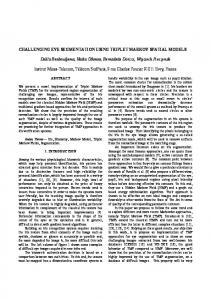
U=u

X=x

Y=y

Gaussian, error ratio 19.12%

Fisher, error ratio 6.34%

Figure 1. Simulated image using TMF model and its corresponding MPM segmentation rseults using Gaussian and Fisher distributions

method is not always numerically tractable, whereas the logmoment is computationally efficient IV.

APPLICATION TO THE SAR IMAGE

We present in this section the results corresponding to an application of the proposed model and its related parameter estimation technique on the simulated and real SAR images. The aim here is to make a comparison in the unsupervised image segmentation context between the use of Fisher distributions and the Gaussian distributions. In the first series of experiment, non stationary simulated triplet Markov Field (ns-TMF), is considered. Thus, we have simulated a non stationary triplet Markov field (ns-TMF), where X takes it values in Ω = {ω 1 , ω 2 } and U takes its values in Λ = {a, b}, which corresponds to the number of stationarities in the simulated image. The class image is then corrupted by the Fisher distribution whose parameters are presented in TABLE 1. Then, the parameters of the model are estimated with the method described in the previous section. Finally, the simulated image is segmented by MPM method. The results of unsupervised segmentation with both Gaussian and Fisher distributions are shown in Figure 1.

TABLE I. Parameters

REAL VALUES OF PARAMETERS AND THE ESTIMATED ONE. CORRESPONDING TO FIGURE 1. Real values 1., 1.

Fisher 0.62, 0.96

Gaussian 1.01, 1.02

2 , α aV2 α aH

1., 1.

0.72, 0.52

0.31, 0.33

α bH2 , α bV2

1., 1.

0.82, 0.61

0.35, 0.32

µ1 , µ 2 M1, M 2 L1 , L2 σ 1 ,σ 2

5., 10.

5.34, 9.77

4.37, 10.38

3., 10.

2.73, 6.87

-

1., 1.

1., 1.05

-

-

-

2.19, 4.96

6.34%

19.12%

α H1 , α V1

Error ratio

As we can see, the suggested technique (ns-TMF+Fisher) performs better than nonstationary TMF combined with Gaussian distribution. However, one can say that the results were foreseeable considering that the experiment represented in this case was fitted to our model i.e. the theoretical one. However the experiment remains interesting in the sense that it provides some knowledge about the robustness of the parameter estimation method suggested here.


Bayard district

Estimated X using Gaussian distribution

Estimated X using Fisher distribution

Estimated U using Fisher distribution

Figure 2. Unsupervised segmentation of Bayard image using ns-TMF+Gaussian, ns-TMF+Fisher

In the second series of experiments, we consider the problem of the real data. The image (2048x2048), shown in Figure 2, represents the Bayard district near Dunkerque, France. This one contains six classes “roads, shadows, buildings, ground and vegetation”. Assuming that we have two stationnarities, the unsupervised segmentation results are depicted in Figure 2. One can say that generally speaking, the results are good; and thus the algorithm proposed could be useful for further applications (registering, 3D reconstruction). The proposed approach has automatically found the salient features of urban landscapes. Among the limits of the proposed approach, we can see that road and shadows have not been clearly distinguished and that there is a class mixing buildings and vegetation (red class). The point is that these features have very close radiometry. Higher level processing should be introduced to deal with this problem (for instance knowledge on building shapes). V.

CONCLUSION

In this paper, we have proposed an original approach based on nonstationary triplet Markov field and Fisher distribution. A comparison between the use of Fisher and Gaussian distributions in the Markovian framework has been done. The main contribution was to tackle the problem of the parameter estimation of the model in order to make unsupervised processing. Experiments testify to the favorable behavior of the method.

Regarding further research, an application of this model to registering and 3D reconstruction could turn out to be promising. REFERENCES [1]

[2]

[3]

[4]

[5] [6]

[7]

[8]

[1]

D. Benboudjema and W. Pieczynski, “Unsupervised image segmentation using triplet Markov fields”, Computer Vision and Image Understanding,” vol. 99, no. 3, pp. 476-498, 2005. J. Marroquin, S. Mitter, T. Poggio, “Probabilistic solution of ill-posed problems in computational vision”, Journal of the American Statistical Association, 82, pp. 76-89, 1987. D. Melas and S. P. Wilson, “Double Markov Random Fields and Bayesian Image Segmentation,” IEEE Transaction on Signal Processing, vol. 50, no. 2, pp. 357-365, 2002. J-M. Nicolas and F. Tupin, “Gamma Mixture modeled with second kind statistics : Application to SAR image processing,” IGARSS, pp. 2489-2491, 2002. P. Pérez, “Markov random fields and images,” CWI Quarterly, vol. 11, no. 4, pp. 413-437, 1998. W. Pieczynski and A.-N. Tebbache, “Pairwise Markov random fields and segmentation of textured images,” Machine Graphics and Vision, vol. 9, no. 3, pp. 705-718, 2000. W. Pieczynski, D. Benboudjema, and P. Lanchantin, “Statistical image segmentation using Triplet Markov Fields,” SPIE’s International Symposium on Remote Sensing, September 22-27, Crete, Greece, 2002. C. Tison, J-M. Nicolas, F. Tupin and H. Maitre, “ A New Statistical Model for Markovian Classification of Urban Areas in HighResolution SAR Images,” IEEE Transactions on Geoscience and Remote Sensing, vol. 42, no. 10, pp. 2046-2057, 2004. G. Winkler, “ Image analysis, random fields and Markov Chain Monte Carlo Methods: a mathematical introduction,” Springer, 2003.