Published in Virtual Reality: Research, Applications & Design, Volume1, Issue 2.
Update Rates and Fidelity in Virtual Environments Rycharde Hawkes1
Simon Rushton2
Research Associate
Research Associate
Martin Smyth3 Undergraduate Student
Virtual Environment Laboratory Department of Psychology University of Edinburgh 7 George Square, Edinburgh, EH8 9JZ 1:
[email protected] (contact author) 2:
[email protected] 3:
[email protected]
Abstract Interaction is the primary characteristic of a Virtual Environment and update rate is normally taken as an index or measure of the interactivity of the system. The speed of many systems is dictated by the slowest component which is often the Computer Image Generator (CIG). It is common for the workload of the CIG to vary and hence the performance of the system. This paper shows how a variable update rate can produce undesirable results. Two solutions to this problem are presented: service degradation and worst-case. In the case of the CIG, service degradation would require the quality of the image to be reduced such that the time taken never exceeds a given deadline. The worst-case technique works by finding the longest time taken to render any view and then uses that as the deadline for completion. The support of predictive methods is one of several benefits of this approach. An implementation of the worst-case technique is described which takes finer control over the CIG than usual and may be applied to many existing systems with little modification. Keywords: Virtual Reality, Computer Image Generators, Real-time Graphics, Update Rate, Tau
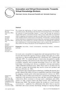
1 Introduction Virtual Environment (VE) systems consist of one or more hardware or software components. Figure 1 shows the basic hardware and software elements of an imaginary driving simulator. The driver uses the steering wheel, brake and accelerator pedals to control their movement through the VE. The environment is presented to the driver via a monitor which is driven by a Computer Image Generator (CIG) and through the force feedback applied to the steering wheel. The pedals and the steering wheel are managed by separate processes or components. The values from these input devices are fed into the dynamics model for the car and a change in position and speed is reflected by instructing the CIG to render a new view of the VE and adjusting the force feedback on the steering wheel. Each component has a particular function and offers a number of services which may be used by the other components. For example, the pedal component's sole service is to provide any interested party the current position of the brake and accelerator. The steering wheel component performs a similar task, in addition it can apply a given torque to the motor linked to the wheel. The consumer of all of these services, and those offered by the CIG, is the 1
Published in Virtual Reality: Research, Applications & Design, Volume1, Issue 2.
dynamics component which must read the current state of the input devices before it can perform its calculations. Only after these have been completed can it instruct the CIG to redraw the display. The time taken to complete a given service has a best and worst case which is dependent not only on the nature of the service, but also on how the other components in the system are performing. Current VE systems are based around a processing cycle that issues service requests which are satisfied as fast as possible. Typically there is always one component that performs worse than the others and becomes a bottleneck. In a distributed system this may be the network interface which is bound by both the speed of the transport medium and the communications protocol being used. In most systems, especially isolated ones, the bottleneck can often be the Computer Image Generator (CIG) which can vary in performance quite drastically depending on visual scene content. This is also the most likely case in our example simulator. In this paper our attention is concentrated on the CIG and how it may be better managed.
CIG
Dynamics
Steering Wheel
Brake & Accelerator
Fig. 1. The basic elements of a driving simulator. Software components are shown in the shaded box on the left and their ties to the real world on the right. Most components take a variable amount of time to complete their processing, so the duration of the processing cycle varies which inevitably means that the displays are updated erratically. Consequently, at the very least, the viewer is presented with incorrect information and, at worst, interaction with the VE is impossible. Adding another component, such as a head tracker, would permit us to head-slave the display such that head movements, when parking for example, would cause a change in the view rendered by the CIG. It would also increase the length of the processing cycle and further destabilise the update rate. In addition, a variable update rate can also present problems if external devices are to be synchronised with the displays. This paper examines the benefits of ensuring that the update rate of VE displays is constant. Two possible approaches to achieving this goal are described and an implementation of one of these solutions used within the Virtual Environment Laboratory (VEL) is presented.
2 Why do we need a constant update rate?
2
Published in Virtual Reality: Research, Applications & Design, Volume1, Issue 2.
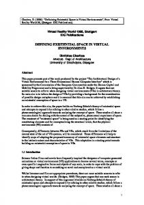
In this section we present an example of the effects that a variable update rate has on interactivity. This is quantified by the application of a visual perception theory. The other benefits of a constant update rate are also discussed. 2.1 Display artifacts Consider a virtual ball moving straight towards you at a constant velocity of 1 m/s. It starts its journey 10 metres from you and you are attempting to catch it. Let us assume that a simulation of this will use a typical variable-rate CIG and a monitor (showing the catchers view) with a refresh rate of 60 Hz. When the ball is in the distance and hence quite small, the CIG manages to generate a new frame 30 times a second. This means that every 2 monitor refreshes a new picture will appear. If the CIG maintains this frame rate then the velocity of the ball will indeed be constant. However, if the CIG should manage to complete it's work within a 60th of a second then the ball's velocity will appear to have doubled to 2 m/s! On the other (more likely) hand, if the CIG's workload takes longer than 33.3 ms to complete and hence only produces a new frame every 3 monitor refreshes, then the velocity of the ball will appear to reduce by 1/3 to 0.66 m/s. If the frame rate was to go up or down each time an image was being rendered1 then catching the ball will be made more difficult. In this case we are likely to see a drop in update rate because as the ball comes towards us, it expands. If the ball was textured and the background blank, this would mean that there are more pixels to fill and hence more work to do. Certainly, we are not seeing what the designer of this simulation wanted us to see. Another more practical example is that of a driving simulator. Given the task of following a vehicle and ensuring that you do not crash into it would be made difficult if the vehicle would seemingly slow down and speed up quite uncharacteristically. 2.2 Judging time-to-contact Lee (1976) presented the Tau theory which suggests that our ability to judge our time to contact with a given target is based upon the rate of expansion of the target on the retina. This may be applied to our ability to catch balls as well as how we control our deceleration, among other tasks (Lee, 1993). The time-to-contact (TTC) of the virtual ball may be expressed as: TTC = Distance / Velocity Fig. 2a shows the TTC assuming that we maintain a constant update rate of 30 Hz which gives us a perceived constant velocity of 1 m/s. The impact of a variable update rate is shown in Fig. 2b. Each time the update rate changes so does the TTC, forcing the catcher to continuously readjust. In this case, the catcher will probably catch the ball because the update rate has slowed down so much that the perceived velocity of the ball at 5 Hz is 0.16 m/s,
1
The word ‘render’ is used in this paper to embrace both of the classical geometrical and rendering stages used to produce an image.
3
Published in Virtual Reality: Research, Applications & Design, Volume1, Issue 2.
making the task trivial. They are unlikely, however, to be using TTC information to help them catch.
Hz
Constant Hz
True TTC
35
12
30
10
25
8
20
6 Seconds
15 4 10 2
5
0
0 10
8
6 4 Distance
2
Actual Hz
Hz
0
Actual TTC
35
12
30
10
25
8
20
6 Seconds
15 4 10 2
5
0
0 10
8
6 4 Distance
2
0
Fig. 2. The effect of update rate on time-to-contact (TTC = distance / velocity): a) with a constant update rate TTC decreases correctly at a fixed rate (top), b) a variable update rate causes a continuous readjustment of TTC (bottom). 2.3 Affects on latency
4
Published in Virtual Reality: Research, Applications & Design, Volume1, Issue 2.
If the time between sampling input devices and updating the display is too long it can contribute to simulator sickness (Pausch et al, 1992). Just how long is too long is not clear, additionally it is not clear whether the systems used provided a constant or variable display update rate. There is evidence to suggest that humans can adapt to a constant degree of lag (providing that it is not too great) after a reasonable period of time, but how effective the interaction is depends on the task being performed. If the lag varies then adaptation is less likely and it is possible that this will add to simulator sickness. 2.4 Predictive techniques There are methods for reducing the impact of lag on the participant. Kalman filters can be used to compensate for the effects of lags within the system (Friedman et al, 1992, Liang et al, 1991, Dunnett et al, 1995). Such filters have been used to predict the movement of 6 d.o.f. sensors attached to parts of the body, e.g. head and hands. In the case of Head-Mounted Displays this means that the CIG can be asked to generate an image of the participant's viewpoint a short while in the future such that the image reaches the display at the right time. The effectiveness of these filters relies on the constancy of the lag and hence the update rate, without it the results of the filtering would be meaningless. If the progression of time happens at a known rate it is also possible to ensure that objects within the VE appear at their correct positions when the image is eventually displayed. This is especially useful when trying to compensate for the single frame delay introduced in double-buffered CIG systems. 2.5 External device synchronisation It may also be desirable to synchronise the VE display with an external data capture system. An example of such a device is the Ober/2™ infra-red eye-tracking system (Permobil Meditech, Inc., Sweden). A lot of effort has been expended by the manufacturers to ensure that a fast, constant sample rate is achieved, to such an extent that the host machine is configured solely for the purpose of controlling the eye-tracker. Sample rates over 1000 Hz may be achieved although 180 Hz is sufficient for tasks monitoring basic eye movements (Permobil, 1993). In order to determine where the participant was looking within the VE display requires the meshing of two data sets, each with a different sample rate. Whilst, on a variable rate system, it would be possible to record the update rate and then fit the eye-tracker data set to this, the result would be an uneven spread of data points over time. With a constant update rate system the eye-tracker rate can be set at a multiple of the update rate which makes meshing much easier and produces a consistent number of data points per second.
3 Variable and fixed rate systems 3.1 The variable rate paradigm A typical simulation processing cycle is: 1. Sample input devices 2. Perform dynamics calculations 3. Update output devices 5
Published in Virtual Reality: Research, Applications & Design, Volume1, Issue 2.
The VE system may consist of many components, both software and hardware. With each component comes a response time, a best and worst case for receiving data, processing it and outputting a result. Exactly where the bottleneck in the system is depends on the nature of the VE or application. Typically the bottleneck is the CIG. This is especially true in low-end systems where the CIG is more (or totally) dependent on the host processor to complete its task. In this case, image generation often has to be scheduled along with input/output device handling and the dynamics calculations. It is also quite typical for the workload of each component to vary. This is especially the case in the CIG where scene complexity may vary drastically (Airey et al, 1990). 3.2 A fixed rate paradigm In order to provide a constant update rate there are two possible approaches: 1. Derive some predictive algorithms that will enable us to determine the workload of each component and thus the system as a whole. 2. Restrict the update rate to the worst-case. Both these methods are working to complete the 3 steps in our simulation cycle before a given deadline. Once this deadline has been met it is recycled and used again for the next VE display update. If we adopt the first approach then we may use the knowledge of each component's performance to degrade the services it offers such that the deadline for each component will be met. Alternatively, we can demand less of the system such that, even in the worst-case, it always meets its deadline. This inevitably means using some components at less than optimum performance. Both of these techniques will now be discussed in further detail. 3.2.1 Service degradation This technique requires a scheduler to determine acceptable time-frames within which each component in the system must complete its calculations. The addition of a scheduler brings us one step closer to a real-time system. Failure to meet a deadline will have different consequences depending on the application. A visualisation may be content with simply providing a lower update rate (albeit constant) whereas a highly interactive application may treat failure to meet the deadline as a fatal condition. These two types are essentially a soft and a hard real-time system respectively. It should be noted that some systems have decoupled the rate at which component services are requested and the update rate of the CIG (Shaw et al, 1992, Wloka, 1993, UVa, 1995). Therefore the simulation may progress as fast as possible, while the CIG generates images as fast as it can. However, CIG performance can still benefit from service degradation. Holloway (1992) draws as much of the visual scene as possible whilst still attempting to meet the deadline. To achieve this the Viper system uses a special feature in the Pixel-Planes PHIGS implementation which allows traversal of a particular part of the database hierarchy to be terminated based on a conditional check of a global flag. In addition, visual objects were given either a high or low priority. High priority objects were always drawn and low priority objects only if time allowed. There is no guarantee that the image will be rendered within the 6
Published in Virtual Reality: Research, Applications & Design, Volume1, Issue 2.
allotted time since Viper uses successive estimates to decide whether it has enough time to render any more and is at the mercy of the underlying operating system (OS). Wloka (1993) proposes a system for time-critical graphics which uses knowledge of the dynamics behaviour of the simulation and a modified graphics database model combined with a scheduler to implement this technique. As Wloka notes, few CIGs support service degradation techniques. The nearest facility that most provide is Level Of Detail (LOD) which attempts to reduce workload by automatically substituting models of different visual complexity based on distance or screen pixel coverage (Reddy, 1995). SGI's IRIS Performer™ goes one step further by providing a mechanism known as dynamic LOD scaling. This provides enough basic information for Performer to decide which combination of LOD models will complete rendering within a certain amount of time (SGI, 1995). The other work done in this area is at the application level as opposed to adding functionality to the CIG. Airey et al use LOD along with other pre-processing techniques to support an adaptive refinement system that trades image realism for speed. Funkhouser and Séquin (1993) use cost and benefit heuristics to determine which LOD model should be used. The cost of an object is the time it takes to render an object with a given LOD using a certain rendering algorithm, whilst the benefit is an estimate of the contribution of the model to human perception. Encouraging results are obtained using this approach, however, even this technique is not sufficient to cope with extreme cases such as changing the view from looking at the sky to looking at a fully textured model of a town. Unfortunately, implementing such a system presents a number of problems. Firstly, most operating systems are not suited to real-time purposes, i.e. they do not provide ways of guaranteeing response times for certain events such as interrupts, Inter-Process Communication and disk I/O. Those real-time systems that do provide such guarantees are often targeted at systems where the system load may be worked out a priori . Clearly a VE system is dynamic and therefore an operating system is required that can cope with changing existing deadlines and the introduction/removal of new tasks and deadlines. 3.2.2 Worst-case operation Establishing what the worst-case is for a given VE can be accomplished by either working out by hand the worst performance of each component or by "exercising" the VE over a period of time. The latter method is very convenient and relatively effortless to perform, however its effectiveness is dependent on exercising the parts of the system that will present the worst performance, either on their own or combined with other components. A major advantage of this approach is that it may be used on existing systems and although scheduling still plays an important part, it is done on a decidedly pessimistic basis. The price paid for this type of predictability is the under utilisation of the available services, which is sometimes quite extreme if there is a large bottleneck in the system.
4 A Virtual Environment Support System (VESS) 4.1 System requirements Our experimental work is in the area of visual perception, requiring us to measure human perception and motor responses which occur in a matter of milliseconds (Hawkes, 1993). To 7
Published in Virtual Reality: Research, Applications & Design, Volume1, Issue 2.
accurately respond to and measure the effects of such responses it is essential to provide an accurate representation of the VE at any instant in time. In addition we must be able to quantify the side-effects of the experimental equipment, record them and take them into consideration when analysing the results. Not only must we be sure that things look and behave correctly, but we also need to be able to say exactly when certain events occurred and for how long, e.g. that the input device was sampled 20 times a second, 10 ms after the last frame was displayed. A case in point is the simple driving simulator we use for some of our work. Input devices that must be sampled include the brake pedal, throttle, gear stick and steering wheel. Values from all the inputs are fed into a dynamics model which calculates the new position and orientation of the car, amongst other variables. It also provides information which is used to adjust the force feedback on the steering wheel and the sound generated by the car.
VEM
VIS
Car Object
AUD Application Level
CIG
Brake, Accelerator, Wheel, etc.
Device Level Eye Tracker
Speakers
Fig. 3. Example configuration of the Virtual Environment Support System.
4.2 System architecture There were three main reasons for not choosing the service degradation solution: 1. The bottleneck in our system is the CIG which does not offer any way of controlling the time spent rendering. 2. The success of this technique relies on the ability to meet application imposed deadlines. However, most operating systems do not guarantee performance and can sabotage the best planned schedule. 3. A general purpose system, whilst desirable, would take an unjustifiable amount of time to implement. Fig. 3 shows the basic components of VESS as they are configured for the driving simulator. The heart of the system is the Virtual Environment Manager (VEM) whose responsibility is to 8
Published in Virtual Reality: Research, Applications & Design, Volume1, Issue 2.
co-ordinate and minimise the lags introduced by the other components. These can be split into two categories: Managers and Objects. The Managers provide services that complement those provided by the VEM whilst the Objects are the consumers of these services. Two common Managers are the Visual Manager (VIS) and the Audio Manager (AUD). VIS provides a set of CIG independent services which are used by both the VEM and the Objects. The VEM controls the update of the visuals (as described later) whilst the Objects may manipulate their own representation. In a similar way, through AUD, background environment sounds are controlled by the VEM and each Object has complete control over its aural properties. The VEM is responsible for advancing simulation time and at the beginning of every time step, each Object is requested to update their state for the specified time. In the case of the Car Object this requires the sampling of all the input devices, performing the dynamical calculations, updating the output devices and changing the relevant visual and aural properties. Once all the necessary Objects have completed their update and the Managers have finished any important outstanding service requests, the displays are updated and simulation time is progressed. For all our simulations, simulation time directly maps to real world time. 4.3 Managing a CIG There are a number of operations and pieces of information that VIS needs to enforce a fixed frame rate in the CIG: 1. Manual control over buffer swapping 2. The time between one display refresh cycle and the next. 3. The amount of time that the rest of the system components need to complete their work for the next simulation update. 4.3.1 Manual buffer swapping This is essential to the task at hand. Double-buffered systems will display the last rendered image until the current one has been finished. At this point the new image is displayed and the next image is rendered into the other buffer. The switch actually happens during the next vertical retrace (or flyback) phase. On displays such as monitors, this is when the electron gun makes its way from the bottom-right corner of the tube (as the viewer sees it) to the topleft, ready to start drawing the next picture. To achieve our goal we must be able to choose which vertical retrace is used. 4.3.2 Inter Refresh Time (IRT) The IRT is the time it takes to draw one picture on the display including the vertical retrace period. For example, say that a 640x480 resolution image is refreshed at 60 Hz. This means that the IRT is 1000 / 60 = 16.66_ms. The refresh rate varies depending on the resolution of the video signal, e.g. an 800x600 pixel image is often refreshed at 72 Hz, and different display devices can handle different ranges of refresh rates.
9
Published in Virtual Reality: Research, Applications & Design, Volume1, Issue 2.
The refresh rate may be provided as a parameter at run-time or, alternatively, this information may be obtained from the CIG. This is the approach we have taken. Each time the CIG generates a vertical retrace it also generates an interrupt which is intercepted by the host machine and the time stored. The next time an interrupt is caught, the time difference is calculated and this gives us the IRT. This technique will only work if the host machine has a clock that can provide nanosecond accuracy and the interrupt latency2 is bounded. The latter point is by no means certain in nonreal-time operating systems such as UNIX and was one of the main reasons we opted for a real-time system (QNX - QNX Systems, Ontario). 4.3.3 Inter Update Time (IUT) The total processing time required for one simulation update (which includes the time VIS and the CIG needs to complete their work) is provided by the VEM. VIS then finds the nearest multiple of the IRT to the given time which gives us the IUT. In other words, the total work time can be expressed as a number of display refreshes. For example, if the IRT is 16.6_ms and the work takes 40 ms, the IUT would be 49.9_ms, i.e. the work may be done within 3 refreshes of the display.
a)
b)
t=0
t=1
t=2
c)
t=-1
t=1
t=0
t=2
Key Refresh cycle Deadline
Calculate state Render new frame Display frame
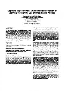
Fig. 4. Simulation cycle scheduling: a) buffer swaps happen at unpredictable times during the next simulation cycle in a variable rate system, b) controlled buffer swapping in a single CPU fixed rate system, c) a multiprocessor fixed rate
2
The time between the interrupt being generated and the process on the host machine being notified of the event.
10
Published in Virtual Reality: Research, Applications & Design, Volume1, Issue 2.
system permits the calculation stage to be done in parallel and in advance of the rendering stage resulting in a faster update rate. 4.4 A comparison of paradigms Fig. 4 shows the various ways of scheduling the work to be done each frame. There are three basic stages: calculate, render and display. 4a shows how these stages fit together in a variable rate system and how they relate to the display refresh cycle. The time at which the frame may be displayed varies and rarely coincides with a vertical retrace, which means that the actual buffer swap happens at sometime during the next cycle. As shown in the diagram, most of the time the calculation stage may progress immediately and by the time this is finished, the buffers have been swapped and the render stage is ready to continue. However, the last complete cycle in 4a shows that it may be necessary for the render stage to wait until the buffers have been swapped. This is because the buffer that will be filled next is currently being displayed. The scheduling of the work in a fixed frame rate system is shown in 4b. The time between the end of the rendering stage and the display will vary depending on how long it takes to render the scene. Pseudo-code for this process is given in Fig 5. Both these examples assume that all work is being done by one CPU. If the image generation can be dedicated to another CPU or the system is equipped with a separate graphics subsystem, then time may be saved by scheduling the calculate and render stages such that they overlap as shown in 4c. This is best achieved by starting the redraw as soon as possible (since it will take the longest time to complete). In order that we are rendering the most upto-date state possible, the calculation stage is done before the end of the previous frame. By performing these two stages in parallel it also means that more time can be spent on the simulation dynamics. Obviously, failure to complete either of these stages before the designated refresh occurs is a system failure. Regardless of technique, it is important to understand how the CIG works and the latency that it introduces into the process since not all CIGs work the same way. For example, an SGI RealityEngine/2™ introduces a one frame latency whilst the Real World Simulation Reality3™ PC card produces a two frame latency. We have used the latter system and to compensate for this latency, state calculations must be done two updates before the image needs to be displayed. This method of controlling double-buffering can be applied to most CIGs with few problems since it utilises existing functionality. It may be necessary, however, for the Application Programmers Interface (API) to be modified to gain access to this functionality. // Step 1: Initialise key variables Calculate IRT Calculate IUT based on totalWorkTime Enable manual buffer swapping displayTime = 0 // Step 2: Synchronise loop with display Wait for refresh
11
Published in Virtual Reality: Research, Applications & Design, Volume1, Issue 2.
// Step 3: Enter main processing cycle While simulation not complete { // Step 3.1: Calculate state displayTime = displayTime + IUT Calculate state of VE for displayTime // Step 3.2: Draw new image but don't display Redraw display // Step 3.2: Display image exactly on time Wait for end of IUT period Swap buffers }
Fig. 5. Pseudo code for the fixed frame rate, worst-case simulation cycle.
4.5 Further improvements It is quite common for the render stage (even in its worst-case) to complete before the time that the display stage needs to run (as shown in Fig. 4c). If this is the case then the start of the state calculation, which includes input device sampling, and the render stage may be put back such that there is even less delay between calculation and display (Fig. 6a).
a)
t=-1
t=0
t=1
t=2
t=23.5
t=24.5
b)
t=21
t=22
t=22.5
t=23
Key Refresh cycle Deadline
Calculate state Render new frame Display frame
Fig 6. Improved simulation cycle scheduling. a) shifting the calculate and render stages to reduce system latency, b) performance profiling permits the increase/decrease of the update rate in a controlled manner. 12
Published in Virtual Reality: Research, Applications & Design, Volume1, Issue 2.
A more advanced technique is the controlled increase or decrease of update rate. It would be possible to detect whether the CIG is capable of going faster, e.g. making the change between 30 Hz and 60 Hz, by maintaining a history of its execution time for each update. If, after a small period of time, this new potential performance was maintained then the other stages could be rescheduled, if possible, and the switch made (Fig. 6b). In a similar way, by monitoring the performance profile, a slow increase in workload could be detected and a decision made to extend the deadline. Once a decision is taken to change the deadline, no further changes must be made for a reasonable period of time, e.g. a couple of seconds, or things would quickly degenerate into a variable rate system. Such an enhancement could also help overcome the fact that the worst-case approach assumes that the environment is quite static and does not cope well with the dynamic creation or destruction of objects. Some multiprocessor CIGs already monitor image complexity to aid in processor loadbalancing. For example, the Reality3™ system, uses knowledge of the changing complexity of each scan-line to predict the load distribution for the next update. With additional functionality in the API, these calculations could be used in the decision-making process. It is true that simple decision-making logic could be flawed by fast increases or decreases in workload, but the potential increase in system fidelity makes it worthy of more investigation. A deadline-based approach also provides the framework for the application of object priority systems within the CIG as well as the VEM. Objects may be drawn, partially drawn or skipped depending on their priority (as in the Viper system). Similarly, the VEM may request a reduced quality service from a lower priority Object to meet the deadline.
5 Conclusion The problem of presenting a temporally correct view of a VE has implications throughout the whole support system architecture. The most efficient technique for achieving this goal is a system whereby each component offers a service whose quality may be tailored to fit the time available for completion. The practicalities of offering such a service are many. The most important (and often the most expensive) component of a VE system is the CIG. Most CIGs provide some form service degradation in the form of LOD but this is insufficient and improvements must be implemented via the API. An efficient VE system must also demand certain guarantees from the underlying operating system such as maximum interrupt latency and context switch times. Sadly, few of the OSs used in today's systems fulfil all of the requirements. Consequently, a less efficient worst-case technique and details of its implementation were presented. Producing successive displays of a VE at a variable rate can be shown to cause interactivity to suffer. The sense of presence in VEs is another area where variable rates may have an effect. In the study performed by Barfield and Hendrix (1995), five different update rates were used to examine the sense of presence. Efforts were made to ensure a constant update rate but it would also be interesting to see the effect that a variable update rate has on presence - which is currently a far more realistic situation. Increasingly, other complex standalone hardware (such as eye-trackers) are being incorporated into VE systems. Without a common time-frame, attempts to synchronise this equipment with a VE system can provide anything from erroneous to useless results.
13
Published in Virtual Reality: Research, Applications & Design, Volume1, Issue 2.
Whilst a constant update rate permits object positions to be calculated into the future, predicting the actions of a human interacting in the VE is another matter. Estimation of the participants head and possibly hand movements may be accomplished using Kalman filtering but there is no way of anticipating what they will do next. Because of this there will always be a latency between human action and displayed reaction with an order of one or two updates. However, it is surely better to base a judgement on a VE whose state is correct for that moment in time, than to base judgements on out-of-date information.
References Airey J., Rohlf J. and Brooks F. (1990) Towards Image Realism with Interactive Updates Rates in Complex Virtual Building Environments. Computer Graphics 24(1): 41-50. Barfield W. and Hendrix C. (1995) The Effect of Update Rate on the Sense of Presence within Virtual Environments. Virtual Reality: Research, Development and Applications 1(1): 3-16. Dunnett P., Harwood R.M., Brookes G.R. and Wills D.P. (1995) Use of a Modified Kalman Filter for a Visually Coupled System Application. Virtual Reality: Research, Development and Applications 1(1): 57-68. Friedmann M. Starner T. and Pentland A. (1992) Synchronisation in Virtual Realities. Presence Teleoperators and Virtual Environments 1(1): 139-144. Funkhouser T. and Séquin C. (1993) Adaptive Display Algorithm for Interactive Frame Rates During Visualization of Complex Virtual Environments. Proceedings of SIGGRAPH ‘93: 247-254. Hawkes, R. (1993) The Virtual Environment Laboratory. Proceedings of the Virtual Reality Systems Conference '93, NY. Holloway R. (1992) Viper: A Quasi-Real-Time Virtual-Worlds Application. Technical Report TR92-004, UNC, Chapel Hill. ftp://ftp.cs.unc.edu/pub/techreports/92-004.tar.Z Lee D.N. (1976) A theory of visual control of braking based on information about time to collision. Perception 5: 437-439. Lee D.N. (1993) Body-environment coupling IN Neisser U. (ed.) The perceived self: Ecological and interpersonal sources of self-knowledge (Cambridge University Press): 43-67. Liang J., Shaw C. and Green M. (1991) On Temporal-Spatial Realism in the Virtual Reality Environment. Proceedings of the 4th Annual Symposium on User Interface Software and Technology: 19-25. Pausch R., Crea T. and Conway M. (1992) A Literature Survey for Virtual Environments: Military Flight Simulator Visual Systems and Simulator Sickness. Presence Teleoperators and Virtual Environments 1(3): 344-363. Permobil Meditech, Inc. (1993) Operating and Installation Manual for the Ober/2 12 bit Parallel System.
14
Published in Virtual Reality: Research, Applications & Design, Volume1, Issue 2.
Reddy M. (1995) A Survey of Level of Detail Support in Current Virtual Reality Solutions. Virtual Reality: Research, Development and Applications 1(2). SGI (1995) IRIS Performer Programmers Guide. Shaw C., Liang J., Green M. and Sun Y. (1992) The decoupled simulation model for virtual reality systems. Proceedings of the CHI'92: 321-328. UVa User Interface Group (1995) Alice: Rapid Prototyping for Virtual Reality. IEEE Computer Graphics and Applications 15(3): 8-11. Wloka M. (1993) Dissertation Proposal: Time Critical Graphics. Department of Computer Science, Brown University, Providence, Rhode Island. CS-93-50.
Acknowledgements Many thanks to Martin Reddy for reading drafts of this paper and providing constructive feedback. This work was undertaken on JCI/MRC Grant G9212693: Visual Control of Steering and the SERC Grant: Optic Constraints for Action.
Biographies Rycharde Hawkes graduated from Coventry Polytechnic with a B.Sc. (Hons) in Computer Science in 1991. The following year was spent as an employee of Real World Graphics working on software development for their range of low-cost, real-time computer image generators. In late 1992 he moved to the Virtual Environment Laboratory at the University of Edinburgh. He is currently also pursuing a PhD part-time, the thesis is entitled "A Software Architecture for Modeling and Distributing Artifical Environments". Simon Rushton is a Research Associate in the Department of Psychology at the University of Edinburgh. His areas of research include support for perception in VEs, and the use of VE technology for the investigation of visual motion perception mechanisms and motion perception function following brain damage. Martin Smyth worked in the VEL during his industrial placement year from Napier University, Edinburgh, 1992-93. One of many projects undertaken was the implemention of the CIG's additional API functionality. He is currently completing his honours degree in Computer Science.
Reality3™ is a trademark of Real World Simulation Ltd, U.K. IRIS Performer™ and RealityEngine/2™ are trademarks of Silicon Graphics, Inc, U.S.A. Ober/2™ is a trademark of Permobil Meditech, Inc, U.S.A.
15