USE OF AN ALTERNATIVE TECHNIQUE FOR ESTIMATING STATOR FLUX IN THE DIRECT TORQUE CONTROL OF INDUCTION MOTORS
Sandro Binsfeld Ferreira, José Felipe Haffner *, Luís Fernando Alves Pereira ** Pontifícia Universidade Católica do Rio Grande do Sul PUCRS - FENG – DEE CEP 90619-900 – Avenida Ipiranga, 6681 Porto Alegre - RS – Brasil e-mail:
[email protected]
* Pontifícia Universidade Católica do Rio Grande do Sul PUCRS - FENG – DEE CEP 90619-900 - Avenida Ipiranga, 6681 Porto Alegre - RS – Brasil e-mail:
[email protected]
Abstract — Direct Torque Control of induction motors is the latest step in motor drives. Its high performance torque control has been seen as a viable industrial sol ution. An alternative method to estimate stator flux and rotor resistance variation in working conditions is proposed together with a simulation environment developed in MATLAB/Simulink. This environment takes into account the dynamic behavior of each individual block making it possible to project and test controlling structures for DTC in an inexpensive way.
** Pontifícia Universidade Católica do Rio Grande do Sul PUCRS - FENG – DEE CEP 90619-900 - Avenida Ipiranga, 6681 Porto Alegre - RS – Brasil e-mail:
[email protected]
TABLE 1 TYPICAL TORQUE AND SPEED PERFORMANCE DATA [6] DC drive with encoder
Flux Vector Control (with Encoder)
DTC
DTC (with encoder)
± 3% ---
± 4% ± 1%
± 4% ± 1%
± 3% ± 1%
Response Time
10..20 ms
10..20 ms
1..2 ms
1..2 ms
Speed Control Static accuracy
± 0,01%
± 0,01%
0,1 %
± 0,01%
0,3 %
0,3 %
0,4 %
0,1 %
Torque Control Linearity Repeatibility
I. INTRODUCTION
Dynamic Accuracy
Compared to induction motors, direct current (DC) motors have a number of disadvantages, such as the restriction of power and velocity due to commutators associated with greater complexity and consequent increased cost of machine maintenance. Such factors have given rise to the search for alternative solutions for driving such motors [1]. The method introduced by Blaschke of controlling field orientation has allowed induction motors to be controlled to a performance equivalent to that obtained with DC motors, although it requires measurement or estimation of velocity [2]. The idea of direct torque control (DTC) formulated by Takahashi (1986) and Depenbrock (1988) introduced a new alternative for the control of asynchronous machines [3][4]. Recent papers such as those of Buja and Casadei [5] and Nash [6] point to the advantages of this technique over the more traditional strategies of scalar and vectorial control, mainly considering the improved torque control performance. Table 1 presents typical results of torque and speed performance for different control strategies [6]. It shows two important aspects of DTC that are: • A torque response better than the other alternatives presented; and, • A speed response comparable to a DC drive, with all the advantages involved in the substitution of a DC motor for an induction one. For DTC method to work properly, two key factors must be observed on its implementation, namely: • Precise estimation of stator flux; • This estimate must be obtained during a time interval so short that it allows the machine control signals to be updated.
The first factor, relating to the quality of the stator flux, is directly affected by variation in machine parameters during its operation, especially at small velocities. For this reason, it is convenient to combine the tasks of parameter estimation and flux estimation. The Kalman-RPE algorithm, Hemerly et al. [7], is based on the use of linear Kalman filtering for estimating the flux together with the Recursive Prediction Error (RPE) method for calculating the Kalman filter gains meanwhile estimating the motor parameters that typically vary during operation. Besides, this algorithm has proved to have a good accuracy at small velocities. The second factor is concerned with the speed of stator flux estimation. The Kalman-RPE algorithm has been shown by Pereira et al. [8] to be sufficiently rapid for vector control of induction motors, and is therefore used in the present paper. To obtain results for estimating fluxes, parameters and DTC control, a simulation environ ment was developed using Matlab®/Simulink [9], conceived so as to reproduce aspects only found in the implementation phase. The induction motor model is assumed to be continuous, the algorithm for estimating the flux and parameters is implemented in a discrete form and the dynamics of additional components, such as encoders and anti-aliasing filters, A/D and D/A converters and inverter, are also taken into consideration. The principal aspects to be considered in this paper are the validation by simulation of the DTC method operating in conjunction with the Kalman-RPE algorithm, and the use of project control tools in Matlab®/Simulink made available through development of the integrated environment.
87
II. DIRECT TORQUE CONTROL - DTC
possibilities of the transistors Sw1 to Sw6. The vectors V0 and V7 are null vectors and correspond to situations in which the switches Sw1, Sw3 and Sw5 are simultaneously closed (V0 ), or open (V7 ).
DTC philosophy is based on hysteresis control of torque and stator flux. Fig. 1 shows a block diagram of this control structure. Switching logic is used to select the stator voltage vector for the inverter (spatial modulation). The purpose of this selection is to produce inverter states that will maintain the torque and stator flux within hysteresis boundaries. Torque Reference
3
K=4
2
K=5
K=6
K=0
K=7
V
_
4
_
_
V =V 0
V1
7
V
5
Re ( α)
_
V
6
Fig. 3: Spatial Vectors represented by switching possibilities
DC
Flux Comparator
AC
B. Switching logic
Estimated fllux
The switching logic used for selecting the spatial vector has the following arguments: • Torque error – through the use of a three-level hysteresis are defined three error possibilities: zero, positive or negative, τ=0, 1 or –1. • Flux error – using a two-level hysteresis are defined two possibilities for flux error: zero or positive, φ=0 or 1; • Spatial vector sector – the spatial sector in which the stator flux lies at the moment under consideration.
Position of keys
Motor Estimated frequency
K=3
Converter Switching logic
Flux
Torque Estimator
K=2
_
Torque Comparator
Reference
K=1
_
V
_
Control by Hysteresis
Hysteresis Window
Im (β)
_
V
DC voltage level
Model Stator current
Estimated velocity
Motor
Fig. 1: Block diagram of DTC.
There are six possible voltage vectors and two null vectors chosen as a function of the errors between reference and estimated values for the torque and flux. The motor model provides an estimate of the present motor state. The flux and torque estimates are used in the spatial modulation whilst the mechanical velocity is used in the external control loop. With DTC implementation, it is possible to achieve a torque response of the order of milliseconds according to results obtained by Buja [5].
C. Control of Torque and Stator Flux The stator flux is controlled by means of variation in voltage input applied to the stator. Neglecting the voltage drop involved in the second term of (2), it is observed that the variation in stator flux is approximately equal to the stator voltage generated by the voltage inverter.
A. Spatial Modulation
r& r r λ s = Vs − Rs .I s
Fig. 2 shows a simplified scheme of the voltage converter. For each of the conduction possibilities of the transistors Sw1 to Sw6 there corresponds a unique representation as spatial vectors. When voltages at the points a, b and c (va , vb , vc) are inserted in (1), the spatial vector VS is obtained. 2π 4π j j s 2 v s = v a + vb e 3 + v c e 3 3
(2)
Equation (3) shows that when the absolute value of the stator flux λs is maintained at a constant level, which can be obtained by hysteresis control, a rapid change in the angle α will result in a rapid response in the electrical torque. τe =
(1)
(
)
r r 3 3 .P . λs × I s = .P . λs . I s . sen( α ) 2 2
(3)
D. Switching strategies.
I
Sw 1
Sw 3
a
b
E
Sw 2
Sw 4
Sw 5
There are two basic strategies for calculating the inverter state vector in the traditional approach where sixlevel switching is used [5]. The first, strategy A, considers that a null vector will be used when it is necessary to reduce the torque, occurring a reduction in the angle between the rotor and stator currents due to the rotor’s inertial braking. The advantage of this strategy is a smaller noise in the torque and a reduced switching frequency. On the other hand, when strategy A is implemented alone it is not possible to operate in the four quadrants for rotation in only one sense is permitted.
c
Sw 6
Fig. 2: Simplified scheme of the Voltage Converter.
Fig. 3 shows the spatial representation of voltage vectors V0 to V7 obtained with the various switching
88
Strategy B, presented at Table 2, uses a voltage vector which generates an increment in torque in the opposite direction to motion. A more rapid torque performance, and operation in all four quadrants, thereby become possible. Alternative B, although making a better torque response possible has the drawback of higher frequency.
where the rotor fluxes are derived from (5), which is a version discretized by Euler’s method of the current model of the induction motor, being Rs the stator resistance; Ls the stator inductance; Rr the rotor resistance; Lr the rotor inductance; Lm the mutual inductance; ωr the rotor angular velocity, σ r = R r L r ,
(
φ=1
φ=0
)
σ = 1 − L2m Ls L r , T is the discretization time; i sα and
TABLE 2 SWITCHING LOGIC STRATEGY B
isβ are the stator currents; (v sα , v sβ ) is the stator spatial
θ(1)
θ(2)
θ(3)
θ(4)
θ(5)
θ(6)
τ =1
v2
v3
v4
v5
v6
v1
τ =0
v7
v0
v7
v0
v7
v0
τ =−1
v6
v1
v2
v3
v4
v5
τ =1
v3
v4
v5
v6
v1
v2
τ =0
v0
v7
v0
v7
v0
v7
τ =−1
v5
v6
v1
v2
v3
v4
vector; θ1 is the rotor resistance and ω(n), ν(n) are Gaussian noises associated with measurement and with the process. T 1 − θ 1 − Tω r ( n ) λ rα ( n + 1 ) λ ( n ) L r rα λ ( n + 1 ) = + T rβ Tω r ( n ) 1 − θ 1 λrβ ( n ) Lr TLm 0 i (n) L θ1 sα ω rα ( n ) r + + ω ( n ) TL i ( n ) 0 m θ sβ rβ 1 Lr
(5)
The measured time derivative of rotor flux is obtained by a discretization of the dynamic equation for rotor flux given by the voltage model presented in [7], i.e.
Obs: θ(1) stands for first sector
III. KALMAN-RPE ESTIMATOR
yr α ( n ) TLr = yrβ ( n ) Lm
The algorithm for estimating rotor flux and resistance proposed by Hemerly et al [7] is shown in Fig. 4.
σL L − s r Lm
vsα ( n − 1 ) isα ( n − 1 ) − Rs + vsβ ( n − 1 ) is β ( n − 1 )
is α ( n ) isα ( n − 1 ) υrα ( n ) + − isβ ( n ) isβ ( n − 1 ) υrβ ( n )
(6)
The prediction error, defined as the difference between the time derivatives of rotor fluxes given in equations (5) e (6), is used as input to the estimation algorithm. It can be seen that this estimation algorithm makes natural use of the two models described, combining the inherent advantages of the current model at low velocities with the advantages of the voltage model at higher velocities [8]. IV. IMPLEMENTING DTC BY USING SIMULINK. The results presented in this section refer to the direct torque control of a velocity servomechanism shown in Fig. 5 . The induction motor parameters used in the simulations are presented in Table 3.
Fig. 4: Block Diagrams of Estimator.
In the block diagram of this figure, the predicted time derivative of rotor flux is denoted by y ˆ ( n) . This variable is obtained by consideration of the following observation process: y rα ( n ) 1 0 λrα ( n ) y ( n ) = + rβ 0 1 λrβ ( n ) 1 0 λrα ( n − 1 ) υ rα ( n ) - + 0 1 λrβ ( n − 1 ) υ rβ ( n )
TABLE 3 INDUCTION MOTOR PARAMETERS
Number of poles System inertia Stator resistance Rotor resistance Stator inductance Rotor inductance Mutual inductance
(4)
89
4 0.062 kg.m 0.728Ω 0.706Ω 0.0996H 0.0996H 0.0969H
The philosophy adopted for the simulation phase and for the analysis of direct torque control performance, was to obtain a set of results as near as possible to those expected in the implementation stage. Therefore, three basic sub-systems were considered as shown in the simulation diagram given in Fig. 5 .
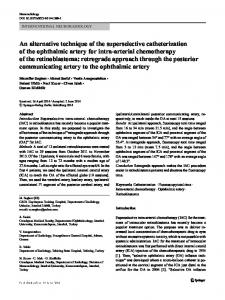
In Fig. 6, we can see that the reference velocity is followed closely while Fig. 7 presents the stator current needed for this velocity reference trajectory to be achieved. Fig. 9 and Fig. 10 show a slight influence of the applied disturbance torque.
The first subsystem is composed of the induction motor frequency converter, of the mechanical load coupled to the rotor axis, and of the anti-aliasing filters. This subsystem is represented in the continuous domain by a set of differential equations that describe its dynamics, and are solved by means of an numerical integration algorithm with integration step of 10µs.
60 Reference Rotor 40
Velocity [rad/s]
20
0
-20
-40
-60 0
0.1
0.2
0.3 0.4 Time [s]
0.5
0.6
0.7
0.5
0.6
0.7
Fig. 6: Reference and real motor velocities.
50 40 30 20 Stator Current [A]
Fig. 5: Simulation environment implemented in Simulink.
The second subsystem is composed of the flux and resistance estimator, the speed controller of proportionalintegral type with proportional gain equals to 100 and integral gain equals to 500. The reference velocity used is shown in Fig. 6. The estimator of flux adopted for implementation in the simulation environment is the Kalman-RPE estimator, because of its performance advantages at low velocities, small sensibility to rotor resistance variations, and because it is only slightly affected by measurement noise. All these blocks are implemented in discrete form since the implementation is achieved by means of software. The interval of discretization used in this subsystem is 1ms.
10 0 -10 -20 -30 -40 -50 0
0.1
Fig. 7: Stator current.
The third subsystem is composed of the direct torque control and of the torque estimator. The switching strategy used is of type B, shown in Table 2. The DTC calculation uses a sampling interval of 50 µs [10]. The maximum switching frequency is limited to 20 kHz. The absolute value of the stator reference current is equal to 0.6 Wb. The motor is operated under a linear variation of up to 100% in the rotor and stator coil resistances in order to verify the application and stability of the estimation algorithm together with DTC strategy. Torque disturbances of 50 N.m were applied to the motor at 0.15s, 0.30s e 0.45s. The motor responded immediately to the requested disturbance torque as it is presented at Fig. 8.
90
0.2
0.3 0.4 Time [s]
Eletromagnetic Torque [N.m] Disturbance Torque [N.m]
100 Reference Torque Torque
50 0 -50 -100 0
0.1
0.2
0.3 0.4 Time [s]
0.5
0.6
0.7
0
0.1
0.2
0.3 0.4 Time [s]
0.5
0.6
0.7
100 50 0 -50 -100
Fig. 8: (a) Eletromagnetic reference torque and resulting torque, and (b) torque disturbance.
Stator Flux [Wb]
1 alpha coord. beta coord.
0.5 0 -0.5 -1 0
0.1
0.2
0.3 0.4 Time [s]
0.5
0.6
0.7
Rotor Flux [Wb]
1 alpha coord. beta coord.
0.5 0 -0.5 -1 0
0.1
0.2
0.3 0.4 Time [s]
Fig. 9: Stator and rotor flux in αβ coordinates.
91
0.5
0.6
0.7
Flux Magnitude [Wb]
0.75 0.7 0.65 0.6 0.55 0
0.1
0.2
0.3 0.4 Time [s]
0.5
0.6
0.7
0
0.1
0.2
0.3 0.4 Time [s]
0.5
0.6
0.7
100
Fase [º]
50 0 -50 -100
Fig. 10: Phase and magnitude of stator flux.
[6] J.N. Nash, “Direct Torque Control, Induction Motor Vector Control Without an Encoder”, IEEE Transactions on Industry Applications, Vol. 33, N.º 2, pp. 333–341, 1997. [7] E. Hemerly, H.A. Gründling and L.F.A. Pereira, “Algoritmo Adaptativo para Estimação de Fluxo em Motores de Indução”, 11 o . Congresso Brasileiro de Automática, São Paulo, Vol. 3, pp. 1119-1124, São Paulo, 1996. [8] L.F.A. Pereira, J.F. Haffner, E. Hemerly, and H.A. Gründling, “Direct Vector Control for a Servopositioner Using an Alternative Rotor Flux Estimation Algorithm”, IECON 98, Aachen, Vol. II, pp. 1587-1591, 1998. [9] L.F.A. Pereira and J.F. Haffner “Ambiente de Simulação para o Desenvolvimento e Validação de Técnicas de Controle Vetorial em Motores de Indução”, V Congresso Brasileiro de Eletrônica de Potência, Foz de Iguaçu, vol. II, pp. 791-796, 1999. [10] C. Lochot, X. Roboam and D. Maussion, “A New Direct Torque Control Strategy for an In duction Motor with Constant Switching Frequency Operation”, EPE95, Sevilla, Vol. II, pp. 431-436, 1995.
Conclusion This article presents an alternative method for estimating stator flux for possible use with DTC strategies. Simulation runs show that the Kalman-RPE algorithm, used together with DTC, is independent of variations in rotor and stator resistance, results in a good response at low velocities even with high torque disturbances. References [1] W. Leonard, “30 Years Space Vectors, 20 Years Field Orientation, 10 Years Digital Signal Processing with Controlled AC-Drives, a Review (Part I)”, EPE Journal, Vol.1, n.º 1, pp. 13-20, 1991. [2] F. Blaschke, “The Principle of Field-Orientation as Applied to the New Transvektor Closed-Loop Control System for Rotating-Field Machine”, Siemens Review, Vol. XXXIX, n.º 5, 217-220, 1972. [3] I. Takahashi and T. Noguchi, “A New Quick Response And High Efficiency Control Strategy of an Induction Motor”, IEEE Trans. On Industry Applications, Vol. 22, n. º 5, pp. 820-827, 1986. [4] M. Depenbrock, “Direct Self Control (DSC) of Inverters-Fed Induction Machine”, IEEE Transactions on Power Electronics, Vol. 3, no 4, pp. 420-429, 1988. [5] G. Buja and D. Casadei, “Tutorial: The Direct Torque Control if Induction Motor Drives”, ISIE’97, 1997.
92