Use of ArchaeoPhases on MCMC outputs extracted from Oxcal Anne Philippe
Marie-Anne Vibet
Universit´e de Nantes, LMJL
Universit´e de Nantes, LMJL
Abstract We give a practical introduction to the package ArchaeoPhases using published data modelled by Oxcal and comment the statistical results.
Keywords: ArchaeoPhases, Oxcal, MCMC samples.
In this tutorial, we considered the same example as Philippe and Vibet (2017) but here the modeling was done with Oxcal (See Ramsey (2009, 2016)). We consider the same model as Bosch, Mannino, Prendergast, O’Connell, Demarchi, Taylor, Niven, van der Plicht, and Hublin (2015). The script is given in the Supplementary material of the paper. The Markov Chains simulated by Oxcal were then extracted to illustrate the use of ArchaeoPhases, version 1.0. This procedure is described in Philippe and Vibet (2017). The results obtained related to the phases are not exactly similar, i.e. there are numerical differences, as the Bayesian model considered by Bosch et al. (2015) with Oxcal cannot be implemented in ChronoModel.
1. First steps with ArchaeoPhases 1.1. Installing the package ArchaeoPhases When R is launched, you need to install (only the first time) the package ArchaeoPhases using the following code : R> install.packages(’ArchaeoPhases’, dependencies = TRUE) R> library("ArchaeoPhases")
1.2. Importing data into R software To import the data file into R, you may use ImportCSV() function. For CSV files extracted from ChronoModel sotfware, there is no need to specify any other parameters than the name of the file (and the path to it). Otherwise, you may change the specification after ”sep=” and ”dec=”. The parameter ”comment.char=” is used to define how comments are written in the file to be imported.
2
ArchaeoPhases: Analysis of Archaeological Phases
1.3. Diagnostic tools The output of any Bayesian modeling is simulated chains, we can check the convergence of these chains using the diagnostic tools given by the package coda. In order to use a function from coda, data as to be transformed in a mcmc.list using the function coda.mcmc. This function as two parameter : the data and the number of parallel chains. Let’s use the dataset called ’KADatesOxcal’, containing the MCMC outpout of the modeling implemented in Oxcal. 10 000 iterations were saved in this file. We will consider that there were 2 chains in order to test the convergence of the Markov chains. R> data(KADatesOxcal) R> Dates_mcmc = coda.mcmc(data = KADatesOxcal, numberChains = 2) Now, we can trace the history plot of each parameter and see whether the chains have reach equilibrium. R> plot(Dates_mcmc[,-1]) A part of the results is given in Figure 1. The Gelman-Rubin diagnostic can also be tested using the following line: R> gelman.diag(Dates_mcmc[,-1]) As all Gelman-Rubin criteria do not take values close to 1, it indicates that the convergence of chains is not reached. This fact is confirmed by the behaviour of the chains in Figure 1-b. In such a situation, it is important to run again the simulation to check if the problem is due to bimodal posterior distributions (which required longer sample to be well estimated) or if the chain has not reached its stationary state. > gelman.diag(Dates_mcmc[,-1]) Potential scale reduction factors:
Ethelruda start.dated.IUP GrA.53000 end.dated.IUP start.Ahmarian GrA.57597 GrA.53004 GrA.57542 GrA.54846 GrA.57603 GrA.57602 GrA.53001 Egbert GrA.54847
Point est. Upper C.I. 1.00 1.00 1.00 1.00 1.01 1.04 1.01 1.06 1.14 1.49 1.05 1.14 1.04 1.06 1.12 1.36 1.23 1.88 1.62 4.59 1.60 4.80 1.61 4.96 1.52 3.99 1.76 5.99
Anne Philippe, Marie-Anne Vibet GrA.57599 GrA.57598 GrA.57544 end.Ahmarian start.UP GrA.57545 GrA.53006 GrA.54848 end.UP start.EPI GrA.53005 end.EPI Multivariate psrf 1.38
1.77 1.80 1.79 1.81 1.04 1.00 1.02 1.05 1.00 1.00 1.04 1.00
6.14 6.35 6.41 6.39 1.16 1.02 1.03 1.08 1.01 1.00 1.07 1.00
3
4
ArchaeoPhases: Analysis of Archaeological Phases
a.
b. Figure 1: Traces and density of several parameters of the Bayesian modeling. (a) Chains show the same stationary distribution. Hence, convergence has been reached. (b) Chains do not show the same evolution. Convergence has not be reached.
Anne Philippe, Marie-Anne Vibet
5
1.4. Examining a series of dates Using the function MultiCredibleInterval, we can estimate the 95% credible interval of each date. R> MultiCredibleInterval(KADatesOxcal, position = c(4, 7:13, 15:18,21:23,26), level = 0.95) which gives the following results : > MultiCredibleInterval(KADatesOxcal, c(4, 7:13, 15:18,21:23,26)) Level CredibleIntervalInf CredibleIntervalSup GrA.53000 0.95 -42613 -41247 GrA.57597 0.95 -41505 -40788 GrA.53004 0.95 -41410 -40687 GrA.57542 0.95 -41434 -40586 GrA.54846 0.95 -41392 -40440 GrA.57603 0.95 -41280 -39907 GrA.57602 0.95 -41319 -39791 GrA.53001 0.95 -41318 -39756 GrA.54847 0.95 -41240 -39394 GrA.57599 0.95 -41247 -39387 GrA.57598 0.95 -41202 -39313 GrA.57544 0.95 -41266 -39270 GrA.57545 0.95 -38655 -37242 GrA.53006 0.95 -36986 -35651 GrA.54848 0.95 -31007 -29789 GrA.53005 0.95 -28515 -27483 The function MultiHPD gives an estimation of the 95% HPD regions of each date (results not shown). R> MultiHPD(KADatesOxcal, c(4, 7:13, 15:18,21:23,26), level = 0.95) All those intervals may be drawn on a graph using the function MultiDatesPlot. The following lines show an example of its use, Figure 2 presents the graph of the credible intervals and Figure 3 displays the graph of a series of HPD regions. R> MultiDatesPlot(KADatesOxcal, c(4,7:13, 15:18,21:23,26), level = 0.95, intervals="CI", title=" 95% CI of Ksar Akil dates") R> MultiDatesPlot(KADatesOxcal, c(4,7:13, 15:18,21:23,26), level = 0.95, intervals="HPD", title=" 95% HPD regions of Ksar Akil dates") Now, the rhythm of occurrence of the dates may be investigated using two functions TempoPlot and TempoActivityPlot.
6
ArchaeoPhases: Analysis of Archaeological Phases
Figure 2: Graph of the credible interval of the series of dates included in Ksar Akil
Figure 3: Graph of the HPD regions of the series of dates included in Ksar Akil
Anne Philippe, Marie-Anne Vibet
7
R> TempoPlot(KADatesChronoModel, position = c(2:17), level = 0.95, title=" Tempo plot") R> TempoActivityPlot(KADatesChronoModel, position = c(2:17), level = 0.95) Figure 4 displays the tempo plot and the activity plot of the site of Ksar Akil. From these graphs, we can see that the highest part of the sampled activity is dated between -45 000 to -35 000 but two dates are younger, at about -31 000 and -27 000.
8
ArchaeoPhases: Analysis of Archaeological Phases
Figure 4: Tempo plot [top] and activity plot [bottom] of Ksar Akil
Anne Philippe, Marie-Anne Vibet
9
2. Analysis of archaeological phases 2.1. Needs for ArchaeoPhases As said in Philippe and Vibet (2017) Section 2, a phase or a group of dates is defined by the date of the minimum and the date of the maximum of the group. Hence, we need to create a file containing those values for each phase using the function CreateMinMaxGroup() as follow: R> KAPhasesOxcal = CreateMinMaxGroup(KADatesOxcal, c(4), name = "IUP") R> KAPhasesOxcal = CreateMinMaxGroup(KADatesOxcal, c(7,18), name = "Ahmarian", add=KAPhasesOxcal) R> KAPhasesOxcal = CreateMinMaxGroup(KADatesOxcal, c(21,23), name = "UP" add=KAPhasesOxcal) R> KAPhasesOxcal = CreateMinMaxGroup(KADatesOxcal, c(26), name = "EPI", add=KAPhasesOxcal, exportFile = "KAPhasesOxcal.csv") Now, a data frame called ”KAPhasesOxcal” is created and contains the minimum and the maximum values of all phases and a CSV file is also created in order to save these values.
2.2. Examining an archaeological phase From the output of the MCMC algorithm, one can estimate the duration of the groups as the value of the maximum - minimum at each iteration. One can also estimate the phase time range as the shortest interval that contains all the dates of the group at a given confidence level (see Philippe and Vibet (2017)). If interested in the summary statistics of the characteristics of a phase / group of dates, use the function PhaseStatistics(). For instance, let’s examine the summary statistics of the phase Ahmarian. attach(KAPhasesOxcal) R> PhaseStatistics(Ahmarian.Alpha, Ahmarian.Beta, level = 0.95) The output of the R console is then : > PhaseStatistics(Ahmarian.Alpha, Ahmarian.Beta, level = 0.95) Minimum Maximum Duration mean -41147.00 -40529.00 618.00 MAP -41119.00 -40888.00 133.00 sd 253.00 642.00 713.00 Q1 -41237.00 -40988.00 112.00 median -41124.00 -40838.00 268.00 Q2 -41010.00 -39952.00 1148.00 level 0.95 0.95 0.95 CredibleInterval Inf -41505.00 -41266.00 0.00 CredibleInterval Sup -40788.00 -39270.00 1921.00 HPDRInf 1 -41484.00 -41689.00 -189.00
10 HPRDSup 1
ArchaeoPhases: Analysis of Archaeological Phases -40760.00 -39301.00 NA NA NA NA
836.00 904.00 1981.00
PhaseStatistics() results in a matrix of several summary statistics according to the marginal posterior density of the minimum, the maximum and the duration of the phase Ahmarian. The default confidence level is 0.95. The following code gives the endpoints of the time range of the phase Ahmarian (the group of dates that constitute the phase Ahmarian) and recall the given confidence level. R> PhaseTimeRange(Ahmarian.Alpha, Ahmarian.Beta, level = 0.95) The output of the console is > PhaseTimeRange(Ahmarian.Alpha, Ahmarian.Beta, level = 0.95) level TimeRangeInf TimeRangeSup 0.95 -41573.00 -39174.00 Function PhasePlot may be used to draw a plot of the marginal posterior density of the minimum and the maximum of a phase on a same graph. R> PhasePlot(Ahmarian.Alpha, Ahmarian.Beta, title ="Characterisation of phase Ahmarian")
The result is shown on Figure 5. Marginal posterior densities of the minimum and the maximum of the phase Ahmarian (curves) are presented with the shortest credible interval (solid line under the curve) at the desired level (default = 95 %) and their mean value (a dot under the curve) using the same color. In addition, the time interval of the phase at the desired level (default = 95 %) is also presented by a solid line above the curves. PhaseDurationPlot draws the marginal posterior density of the duration of the phase with its shortest credible interval and its mean value. By default, the confidence level is fixed at 0.95 and graphs are in color but these details may be changed. Figure 6 displays the result. R> PhaseDurationPlot(Ahmarian.Alpha, Ahmarian.Beta, title ="Duration of Phase Ahmarian")
Anne Philippe, Marie-Anne Vibet
11
Figure 5: Plot of the marginal posterior densities of the minimum and the maximum of phase Ahmarian
Figure 6: Plot of the duration of phase Ahmarian
12
ArchaeoPhases: Analysis of Archaeological Phases
2.3. Examining the succession of two phases Let’s use for this example the succession of phases IUP and Ahmarian. As these phases are in temporal order, we can estimate, if it exists, the gap (or hiatus) and the transition interval between both phases (see Philippe and Vibet (2017) Section 2 for more details). To test if there exists a gap at 95% between these successive phases, let’s use the function PhasesGap. R > PhasesGap(IUP.Beta, Ahmarian.Alpha, level = 0.95)
> PhasesGap(IUP .Beta, Ahmarian.Alpha, level = 0.95) level HiatusIntervalInf HiatusIntervalSup "0.95" "NA" "NA" This code gives the endpoints of the gap interval between both phases. The default confidence level is 0.95. Now, to estimate the transition interval at 95% between these successive phases, let’s use the following line: R> PhasesTransition(IUP.Beta, Ahmarian.Alpha, level = 0.95) And the result is: > PhasesTransition(IUP.Beta, Ahmarian.Alpha, level = 0.95) 0.95 TransitionRangeInf TransitionRangeSup 0.95 -42572.00 -40751.00 At 95%, the transition between these two phases starts at -42 572 and ends at -40 751. All these pieces of information may be illustrated on a graphic using the function SuccessionPlot(). Figure 7 presents the resulting graph. R> SuccessionPlot(IUP.Alpha, IUP.Beta, Ahmarian.Alpha, Ahmarian.Beta, level=0.95)
Anne Philippe, Marie-Anne Vibet
13
Figure 7: Plot of the succession of phase IUP and phase Ahmarian and 95% intervals. Curves represent the densities of the minimum and the maximum of each phase. The oldest phase is drawn in blue, the youngest phase in violet. As there is only one date in phase IUP, the minimum of the phase equals the maximum of the phase. Hence, only one density can be seen. One-coloured segments correspond to the time range of the phase of the same color, two-colored segments correspond to transition intervals or to gap ranges. A cross instead of a two-colored segment means that there is no gap range at the desired level of confidence.
14
ArchaeoPhases: Analysis of Archaeological Phases
2.4. Examining a series of phases We may also be interested in a series of phases, as for instance the following phases of Ksar Akil: IUP, Ahmarian, UP and EPI. We could, for example, wish to know the time range of these different phases, or we could want to draw the different minimums and maximums on a same graph. We could also wish to know the credible interval of all minimums. To do that, the ”Multi” functions are available. For data extracted from ChronoModel software or using the function CreateMinMaxGroup(), only the vector of positions of all phases’ minimums are needed, as the maximums are the column next to the minimums’. By default, the argument of position_maximum is equals to position_minimum + 1. Otherwise, the vector of positions of the phases’ maximums should be specified. For example, let’s estimate the time range of phases IUP, Ahmarian, UP and EPI, whose minimums are respectively in position 2, 4, 6 and 8. The following line gives the endpoints of the time range of phases whose minimums are in position 1,3,5 and 7. R> MultiPhaseTimeRange(KAPhasesOxcal, position_minimum = c(1,3,5,7))) By default, the argument of position_maximimum is equals to position_minimum + 1. > MultiPhaseTimeRange(KAPhasesOxcal, position_minimum = c(1,3,5,7)) Level TimeRangeInf TimeRangeSup IUP.Alpha IUP.Beta 0.95 -42599 -41231 Ahmarian.Alpha Ahmarian.Beta 0.95 -41573 -39174 UP Alpha UP.Beta 0.95 -38617 -29790 EPI.Alpha EPI.Beta 0.95 -28515 -27482 Phase ”EPI” whose minimum output is in column 7 has a time range = [-28 515, -27 482] at a confidence level of 95% and the phase ”IUP” whose minimum output is in column 1 has a time range = [-42 599, -41 231]. The function MultiPhasePlot() generates a plot presented in Figure 8 that illustrates the characteristics of these phases. Curves represent the densities of the minimum and maximum of each phase. One-coloured segments above the curves correspond to the time range of the phases. Characteristics of a phase (minimum and maximum densities, time range) are drawn using the same color. When a group is defined by only one date, then the minimum equals the maximum date of the group. Hence, in that case, only one curve is presented.
Anne Philippe, Marie-Anne Vibet
15
Figure 8: Plot of the series of Ksar Akil’s phases and their associated time range at 95%. The marginal posterior densities of phase IUP are drawn in purple, those of phase Ahmarian are in ligth blue, those of phase UP are in red and those of phase EPI are in light green. As there is only one date in the phases EPI and IUP, the minimum and the maximum of these phases have the same value at each iteration. Hence, we can see only one curve for each of these phases. Time ranges are displayed by segments above the curves of the same color as the densities of the phase.
16
ArchaeoPhases: Analysis of Archaeological Phases
2.5. Examining a succession of phases in temporal order We may also be interested in a succession of phases. This is actually the case of the succession of IUP, Ahmarian, UP and EPI that are in stratigraphic order. Hence, we can estimate the transition interval and, if it exists, the gap between these successive phases. This may be done using the following code : R> MultiPhasesGap(KAPhasesOxcal, position_minimum = c(1,3,5,7)) R> MultiPhasesTransition(KAPhasesOxcal, position_minimum = c(1,3,5,7)) For these functions, the order of the phases is important. The vector of positions of the minimums should start with the minimum of the oldest phase and end with the one of the youngest phase. For data extracted from ChronoModel or using the function CreateMinMaxGroup(), the vector of positions of the phases’ maximums is deduced from the vector of the minimum. For other data, this vector should be specified. > MultiPhasesGap(KAPhasesOxcal, position_minimum = c(1,3,5,7)) Level HiatusIntervalInf HiatusIntervalSup IUP.Beta & Ahmarian.Alpha "0.95" "NA" "NA" Ahmarian.Beta & UP.Alpha "0.95" "-39144" "-38660" UP.Beta & EPI.Alpha "0.95" "-29790" "-28522" > MultiPhasesTransition(KAPhasesOxcal, position_minimum = c(1,3,5,7)) 0.95 TransitionRangeInf TransitionRangeSup IUP.Beta & Ahmarian.Alpha 0.95 -42572 -40751 Ahmarian.Beta & UP.Alpha 0.95 -41241 -37334 UP.Beta & EPI.Alpha 0.95 -30997 -27482 At a confidence level of 95%, there is no gap between the succession of phases IUP, Ahmarian and UP, but there exists one of 1 268 years between phase UP and phase EPI. The function MultiSuccessionPlot() draws the characteristics of such a succession. Figure 9 presents the resulting plot. R> MultiSuccessionPlot(KAPhasesOxcal, position_minimum = c(1,3,5,7), title = "Ksar Akil - Succession of phases: IUP, Ahmarian, UP, EPI ") In that plot, curves represent the densities of the minimum and maximum of each phase. When a group is defined by one only date, the minimum equals the maximum date of the group. Hence, in that case, only one curve is presented. Segments above the curves correspond to time range of the phase associated to a level confidence of 95%. Two-coloured segments correspond to transition interval or to the gap range associated to a level confidence of 95%. A cross instead of a two-coloured segment means that there is no gap between the succession of phases at the desired level of confidence.
Anne Philippe, Marie-Anne Vibet
17
Figure 9: Plot of the succession of phases from Ksar Akil. The characteristics of phase IUP are drawn in red, those of phase Ahmarian are in light blue, those of phase UP are in purple and those of phase EPI are in light green. Again, as there is only one event in the phases EPI and IUP, the minimum and the maximum of these phases have the same values at each iteration. Hence, we can only see one curve for each of these phases. Time range are displayed by segments above the curves. Two-coloured segments correspond to transition interval or to the gap range associated to a level confidence of 95%. As there are no gaps at 95% between phases IUP and Ahmarian, a cross is drawn instead.
18
ArchaeoPhases: Analysis of Archaeological Phases
2.6. Summary We can summary the characteristics of the different phases of Ksar Akil, using the data published by Bosch et al. Bosch et al. (2015) and the modeling done with Oxcal, by the following table : Phase IUP Ahmarian UP EPI
Time Inf -42 599 -41 573 -38 617 -28 515
range Sup -41 231 -39 174 -29 790 -27 482
Transition range Inf Sup NA NA -42 572 -40 751 -41 241 -37 334 -30 997 -27 482
Gap range (if it exists) Inf Sup NA NA NA NA -39 144 -38 660 -29 790 -28 522
Table 1: Results associated with a level of confidence at 95%
References Bosch MD, Mannino MA, Prendergast AL, O’Connell TC, Demarchi B, Taylor SM, Niven L, van der Plicht J, Hublin JJ (2015). “New Chronology for Ksˆar Akil (Lebanon) Supports Levantine Route of Modern Human Dispersal into Europe.” Proceedings of the National Academy of Sciences, 112(25), 7683–7688. doi:10.1073/pnas.1501529112. Philippe A, Vibet MA (2017). “ Analysis of Archaeological Phases using the CRAN Package ArchaeoPhases.” Working paper or preprint, URL https://hal.archives-ouvertes.fr/ hal-01347895. Ramsey CB (2009). “Bayesian Analysis of Radiocarbon Dates.” Radiocarbon, 51(1), 337–360. Ramsey CB (2016). contents.html.
Oxcal 4.2.
URL http://c14.arch.ox.ac.uk/oxcalhelp/hlp_
Affiliation: Anne Philippe Universit´e de Nantes, Laboratoire de math´e matiques Jean Leray 2, Rue de la Houssiniere, 44000 Nantes, FRANCE E-mail:
[email protected] URL: http://www.math.sciences.univ-nantes.fr/~philippe/info.html Marie-Anne Vibet Universit´e de Nantes, Laboratoire de math´e matiques Jean Leray 2, Rue de la Houssiniere, 44000 Nantes, FRANCE E-mail:
[email protected]