Use of conditional probability networks for environmental monitoring

Use of conditional probability networks for environmental monitoring by H. T. Kiiveri CSIRO Mathematical and Information Sciences, Private Bag, Wembley, WA 6014, Australia email: [email protected]

and P. Caccetta School of computing, Curtin University of Technology, Bentley, WA 6102, Australia email: [email protected] and F. Evans CSIRO Mathematical and Information Sciences, Private Bag, Wembley, WA 6014, Australia email: [email protected]

Running head: Conditional probability networks and environmental monitoring

Use of conditional probability networks for environmental monitoring

Abstract Causal or conditional probability networks (CPNs) are shown to provide a natural framework for combining a time sequence of classified satellite images with other maps for environmental monitoring. The key features of CPNs are described by way of application to an example involving the monitoring of salinisation of farmland over time using satellite images and an ancillary data set derived from a digital terrain model. It is shown CPNs can be used to improve mapping accuracies by incorporating knowledge about the spatial and temporal variation of the map classes of interest. The methods provide a practical solution to the challenging problem of mapping and monitoring salt in farmland. The representation and propagation of uncertainty within this framework is discussed, as well as the spatial and temporal prediction of images and maps.

2

1. Introduction This paper considers the problem of using multiple satellite images in conjunction with other maps to monitor the environment. The generic problem is one of integrating multiple sources of data, which have differing levels of uncertainty associated with them, to produce output map products with improved accuracy. We want to do this in a way which allows the assessment, representation and propagation of uncertainty through the process.

A typical problem might involve the use of four satellite images recorded at different times with 1 or 2 ancillary maps or images. Ancillary data sets are used because the satellite sensor is not capable of distinguishing some ground features sufficiently accurately on its own. For thematic mapper (Landsat TM) satellite data, each image can be of the order of 8000 by 8000 pixels with the pixel size being resampled to 25 metres for consistency with other maps. For each pixel, there are 6 commonly-used bands (ie the thermal band is not used). There are a total of about 25 grey scale images involved in the analysis at various stages(e.g. 6 bands by four dates plus a single band landform image) and a data storage and handling requirement of the order of several gigabytes. Given this, computational feasibility is an issue to consider when we deal with this type of data.

The objectives of this paper are (i ) by way of example, provide an overview of conditional probability networks or Bayesian Expert Systems (see Jensen, 1993) and (ii) show how CPNs provide a natural and elegant solution to the data integration problem mentioned above, both in terms of handling the large volumes of data, and the uncertainties inherent in producing the final output products. We also show that CPNs can make use of knowledge about temporal and spatial variations of map classes of interest to improve mapping results.

Section 2 discusses the issues of positional and attribute uncertainty in maps relevant to the salinity mapping problem, while Section 3 contains an overview of CPNs. This overview is built around an example involving the monitoring of salinisation of farmland, as a result of long-term clearing of agricultural land, in Western Australia. In Section 4, we discuss the use of CPNs for interpolation and extrapolation of maps, both spatially and temporally. Section 5 gives detailed results for a CPN designed to map salinity over time in a study area.

3

2. Attribute and locational uncertainty To use satellite images for environmental monitoring requires that the images be accurately rectified to a common map grid so that changes in map classes are due to actual changes on the ground and not location errors. It is useful to calibrate the images to like values (i.e chose a reference image and convert the other years image values to the reference image values ), see Furby et al (1999). The calibration of the images ensures that areas which are relatively stable over time have approximately the same colours in image displays. Following these steps, a maximum likelihood classification (Richards, 1986, or Campbell et al., 1984 ) is performed to identify and map classes of interest on the ground. Details for the data to be used here are given in Evans (1996). The results of the classification process are a set of posterior probabilities at each pixel which indicate the relative certainty in the class label for each pixel, assuming that the pixel actually belongs to one of the classes. Hence, for each class in a classified image, we have a spatially-varying probability surface which represents the relative attribute uncertainty. In these surfaces it should be noted that a probability of one does not necessarily imply that the label is correct, i.e. the class label produced by the classifier is not the same as the true label..

We use the term "hard" for maps in which a specific label is assigned to each pixel and "soft" for maps where the probability of a class is recorded at each pixel. Note that CPNs easily handle both types of maps. Soft maps will form the inputs in the CPN example to be discussed later. This is a new feature of using CPNs with maps.

Figure 1 illustrates a "hard" salt / not-salt map produced from a satellite image which ignores attribute uncertainty. Its associated “soft” maps, one for each class, are also displayed. In general, attribute uncertainty results in as many spatially varying probability maps as there are classes, although one is redundant due to the constraint that the probabilities at each pixel sum to one.

[insert Figure 1 about here]

In addition to attribute uncertainty, classified satellite images also exhibit positional uncertainty since the process of assigning ground coordinates to a satellite image (rectification) is prone to error. In the case of Landsat TM data, a rectification error within plus or minus one pixel (30 metres) is considered acceptable. To see how positional and attribute uncertainty combine here, consider Figure 2 below, where the numbers are obtained from the posterior probabilities for a particular class in a classified image. From Figure 2 the centre pixel in grey has a value of 0.5 representing a significant uncertainty in the salt class label (say) at that pixel. However, as a result 4

of positional error, if there had been a row shift of one pixel, the uncertainty value would actually be 0.6 or 0.1. Similarly if there had been a column shift of one pixel then the value would have been either 0.2 or 0.7. Since we do not know which shifts may have occurred, to combine positional and attribute uncertainties we should weight the possible values in Figure 2 by the probability of the various shifts and compute a local weighted average for each pixel (for more details see the Appendix and Kiiveri, 1997b). Note that the weights may vary spatially. Figure 3 shows an example of the blurring effect of positional error on the attribute uncertainty for the salt class in a subset of a classified image.


Closer inspection of Figure 3 reveals features (lines and paddocks) which are indicated as having a high probability of being salt-affected but which expert interpretation would ascribe to roads and bare paddocks. In the analysis below, this type of image forms only one source of evidence, and much like human witnesses, we can have high certainty about a class in a particular location but still be wrong. Another way of saying this is that the label from the classified satellite image is not the same as the true land cover since different ground cover classes ( e.g. roads, bare ground and salt) may have very similar spectral signatures. In the following, other sources of information will be used to help distinguish classes of interest and produce more accurate output maps.


3. Conditional Probability networks A conditional probability network is conveniently represented by a graph which provides a concise description of the model and the parameters needed to use it ( see Jensen ,1996) and the references therein. The main features of CPNs will be described by way of a specific example, which will then be applied to the salinity monitoring problem in Section 5. Note that in the following, the term image will also be used to refer to a (soft) raster map.

Consider the graph in Figure 4, which represents an example of a CPN. In the graph, squares denote images which are observed (available as data) while the circles denote images which are unobserved (not available as data). The nodes of the graph, represented by circles or squares, are joined by arrows which define directions of "influence". They can be thought of as defining parentchild relationships with parents influencing their children. In Figure 4, C89, C90, C93, C94 denote classified satellite images for the years 1989, 1990, 1993 and 1994 respectively. These images 5

consist of "soft" classified land cover classes (one of which is salt) which will be specified later. The images T89, T90, T93 and T94 are unobserved images of what is actually present on the ground in the years 1989, 1990, 1993 and 1994 respectively (i.e. “true” images). They have the same classes as the classified satellite images. We want to know these; however, apart from ground truthing at limited study sites, we do not have direct observation on these images. Finally, LFP is a landform image identifying hilltops and valley floors. This data set is relevant since it is known that salt tends to occur in valley floors.

We will use the model to predict the true images on the basis of the sequence of classified satellite images and the landform image.


The CPN can be interpreted as follows. The landform image LFP influences (or provides information about) T89; LFP and T89 influence T90; LFP and T90 influence T93; and LFP and T93 influence T94. In other words, the landform and previous ground cover influence the following years ground cover. Similarly, the true images at each date influence the corresponding classified satellite images.

Associated with each node of the graph is a table of (probabilistic or uncertain) rules which determine how the parents influence the children. These tables, in association with the graph, can be used to define a factorisation of the joint distribution of the nine images in the model, see Jensen, 1996, and Kiiveri and Caccetta, 1998. At each pixel, if the images C89, C90, C93, C94 and T89, T90, T93, T94 each has six classes and the LFP image has 2 classes, then there are 2 x 68 ≈ 3.3 million possible class combinations. In the worst case-scenario, we would have to specify a probability for each of these combinations. However, by specifying the model with the graph of Figure 4 we can define values for all these combinations by specifying only 311 rules and their associated uncertainties. The specification of the tables of probabilistic rules required by the CPN will be discussed in Section 3.2 below.

We have chosen the graph of Figure 4 as an intuitively reasonable structure to illustrate the use of CPNs. Of course, other graphs with more arrows could be used. In practice, the selection of an appropriate graph is an important issue and can be done by interviewing experts in the subject matter, by fitting models to a large sparse contingency table (Badsberg,1992) or a combination of both. Another alternative is to choose a model by minimising prediction error on a validation set of 6

ground-truth data. There is also the need to bear in mind computational complexity when we deal with large data sets.

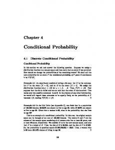
For illustrative purposes, consider the case when all the maps in Figure 4 are binary. In this case, Figure 5 shows some of the probability tables required by the model. In general, each node has an associated table and each table gives an exhaustive list of the class combinations possible for the child node and its parents. A count n and a (conditional) probability p is given for each combination. We will refer to n later. If the table has a dotted line, then the probability of the child node is conditional on the particular class combination of the parents. For example, in Figure 5 for the LFP node, we have a probability 0.17 of a pixel being in a valley, and probability 0.83 of a pixel being on a hill. For the T90 node, the probability of a pixel not being salt (affected) in T90 given that it is in a valley and was not salt affected in T89 is 0.70. For the binary case, there are 29 = 512 possible class label combinations at each pixel. This particular model gives probabilities for all of these in terms of only 23 independent probabilistic rules.


Once these tables of probabilities (uncertain rules) have been specified, we can infer rules which have not been directly specified (e.g. for the class labels in the true maps given the class labels in the observed maps). Efficient algorithms for doing this in real time are given in Lauritzen and Spiegelhalter(1988). An illustration of this is given in Table 1 below. In the table v denotes valley, s - salt affected and ns - not salt affected. These rules are then used to make predictions about the unobserved, true maps.

LFP C89 C90 C93 C94 T89 v s s s s s v s s s s ns v s s s ns s v s s s ns ns . . . 6 ( 2 = 64 possible combinations)

p .999 .001 .997 .003

Table 1: Example illustrating a list of conditional probabilities (uncertain rules) derived from a CPN model for the true classes in the unobserved map T89 given the class combinations in the observed maps 7

3.1 Spatial dependence and CPNs The use of CPNs for integrating image data appears to have been pioneered by Caccetta et al. (1995) and Caccetta (1997). The standard approach involves applying the usual CPN calculations (Lauritzen and Spiegelhalter, 1988 ) independently at each pixel. Other examples which can also be fitted into this framework can be found in Strahler(1980), Hojsgaard et al. (1997) and Stassopoulou et al (1998). For this case (treating pixels independently), the probability tables are kept constant from pixel to pixel and no neighbouring information is used in the calculations, effectively ignoring spatial dependence. Useful results can be achieved with this method, see Caccetta et al. (1995), however improvement in output maps can be obtained by allowing for spatial dependence in the images. A novel and efficient algorithm for handling spatial dependence in CPNs was described in Caccetta(1997). Theoretical results are given in Kiiveri and Caccetta (1996, 1998), using Markov random field models such as in Geman and Geman (1984). One way of representing the model for spatial dependence is to augment the graph of Figure 4 with additional nodes as in Figure 6. At each pixel, each of the images N89, N90, N93 and N94 contain information such as the numbers of neighboring pixels in each different class. The idea is that classes tend to cluster together so that knowledge of neighbouring classes provides information about the class at the pixel of interest. To implement such a model requires, for each pixel, the specification of a set of neighbouring pixels and the specification of spatial and temporal rules. In the present example, the neighbours of a pixel are taken to be the eight nearest neighbours. This neighbourhood was chosen to keep the computations manageable. Larger neighbourhoods can also be defined. A simple, but useful, set of spatial and temporal rules can be obtained through a combination of purely temporal and purely spatial rules. For example, in Figure 6, for T90 we can have probabilistic rules of the form: Probability of salt at a pixel in 1990 is proportional to the probability of salt given landform and salt status in 1989 multiplied by the probability of salt given the number of nearest neighbours which are salt affected. For more details, see Caccetta(1997) and Kiiveri and Caccetta (1998). Transition probability tables can be made to vary spatially and in fact we do this when necessary (i.e when regions appear markedly different in the TM scenes). One way to achieve this would be to define the region under consideration into zones and estimate probability tables separately in each zone. A simple model for this could be represented in Figure 6 by adding another vertex corresponding to an image (map) of zones with arrows pointing to the circles.

8

It should be noted that by augmenting the CPN graph as in Figure 6, existing code for doing CPN calculations is easily modified to handle the case of spatial dependence. With modified code, the production of output maps requires several passes( iterations) through the data. [insert Figure 6 about here] 3.2 Parameter estimation A natural question to ask at this point is: How are the probability tables required by the method obtained ? Some possibilities are: 1. Ask someone who knows e.g. interview experts in the field of application; 2. Estimate the probabilities from the data. In this paper, we will use a combination of 1 and 2. We give an overview of the method in the independent pixel case without going into too much technical detail. For the case of spatial dependence, estimates from the independent pixels case can be combined with spatial rules derived from a simple Markov random field model, see Kiiveri and Caccetta (1996, 1998). First we will assume that all images in the model are observed (e.g. restricted to sufficiently large training areas). This will provide the basis for the calculations in the case when some of the images are unobserved. Following this, we will deal with the real life situation when some of the images are unobserved. When all of the images are observed, to compute the tables as described in Figure 5 requires the computation of the relative frequencies of pixels with attributes defined by the classes (labels) of parent and child nodes. To do this a straightforward counting of the number of pixels with a specific combination of parent and child values is required. Figure 5 illustrates the tables of counts n needed for computing the probability tables from the image data. Note that for the table associated with the landform node LFP, we have 10012 pixels in valleys and 48878 pixels on hills. Similarly, for the table associated with the node T90, we have 16460 pixels in a valley which were not salt-affected in 1989 and not salt-affected in 1990. For each table, given the numbers of pixels with a given combination of class labels, we can compute relative frequencies to obtain the probabilities required. This is done by choosing the count for a particular row, summing counts with the same combination of classes on the left hand side of the dotted line and dividing the first count by the total count. For example, for the table associated with T89, the probability of not being salt-affected in 1989 given the pixel was in a valley is 24092/(24092+6404) =0.79.

9

The case when some images are unobserved (i.e Figure 1) can be handled by the EM algorithm (see Dempster et al (1977) ; Caccetta et al. (1995); and Caccetta,(1997). Basically the algorithm proceeds as follows. 1. Provide initial guesses for the probability tables required. 2. Calculate expected frequencies in the tables of counts needed given the observed images and the current estimates of the probability tables i.e. predict missing counts due to the images not being observed using current probability tables. For example, in Figure 5, the counts in the table associated with T89 can not be computed directly because the classes for T89 are unknown. However the expected values of these counts given the observed data and the current values of the probability tables can be computed. 3. Calculate relative frequencies in the same way as for the all-observed case to update the probability tables i.e. act as if the expected values were actual counts. 4. Repeat 2 and 3 until convergence. This type of procedure converges to sensible estimates (see Dempster et al. 1977). However, some care needs to be taken with models which have unobserved images. Sometimes there is insufficient information in the available images to estimate all the probabilities required uniquely. In this case the algorithm will still converge but there will be a continuum of solutions which will be equally valid i.e. some probabilities are not identifiable. If this is the case, information about some of the probabilities must be supplied from elsewhere. For the example in this paper, we can show that there is sufficient information in the observed images to estimate all the required probability tables. Several different starting values should be used to check for multiple solutions to the estimation problem. Once the probability tables have been estimated by the EM algorithm we can use the CPN to predict values of the true (unobserved) images.

4. Applications of CPNs Having defined a CPN and estimated its parameters, there are a number of interesting and useful outputs which can be produced. We illustrate these for the example in Figure 4.

10

Firstly, we can propagate uncertainties, whether attribute or positional or both, in the input maps C89, C90, C93, C94 and LFP to produce hard or soft true output maps T89, T90, T93 and T94. Secondly, we can make predictions by extrapolation and interpolation. In Figure 7, images with dotted nodes can be predicted. To illustrate, from the model of Figure 4 it is possible to estimate the five-year transition probabilities for classes in 1994 given those in 1989 and the landform categories. Assuming that these have been relatively constant over time, these values can be used to predict images five years backwards and forwards in time ie T84 and T89 in Figure 7. Note, however, for the example analyzed in this paper transition probabilities are not assumed relatively constant and are allowed to vary with time. The assumption of relatively constant transition probabilities is simply one way of obtaining transition probability tables for predicting at times other than those for which data is available. [insert Figure 7 about here] To illustrate temporal interpolation, consider the nodes T91 and T92 in Figure 7. Assuming that the one-year transition probability tables have been relatively constant, we can use the existing tables associated with T90 and T94 to infer values for the tables associated with T91 and T92. Given these tables it is possible to predict the true maps T91 and T92. Thirdly, CPNs for images handle missing data in a natural way. If data in any of the classified satellite images C89, C90, C93 and C94 are missing due to cloud cover, for example, predictions of the true maps in the areas affected by cloud cover will still be made on the basis of all available data i.e. we condition on all the available data at a pixel to make predictions. This means that spatial predictions (interpolations) within the extent of an image are possible. An example of this is given in Kiiveri (1997a).

5. An example We report the results of using the CPN defined by Figure 4 on a 1045 by 1045 pixel study area called Ryans Brook. The satellite imagery has been resampled by cubic convolution to a pixel size of 25 metres. Four classified Landsat TM satellite images collected in the spring of 1989, 1990, 1993 and 1994 are available. Each image was classified into six classes: salt; mixed salt and bare (spectrally inseparable salt and bare cover, mainly bare); bare ground; remnant vegetation; agriculture; and water. The landform image has two classes, hills and valleys ( we could also have finer distinctions such as slopes etc). Each of the images C89, C90, C93, C94 and LFP were input as soft maps i.e. class label attribute uncertainty was represented. Thus we had 5 sets of spatially 11

varying probability maps for input data. Previous work by Furby et al. (1995) has demonstrated that salinity can be mapped and monitored using easily available data sets such as those mentioned above. Note that in any one satellite image it can be difficult to distinguish some bare ground from salt. We will use the combination of a time series of images and landform to improve the mapping accuracy. To do this, we draw on the notion that salt at a particular location tends to be stable over time, while bare ground is less consistent from year to year. We also use the knowledge that salt tends to occur in valleys with a higher probability than in other landform types. Values for the following probabilistic rules were fixed beforehand: (i)

Probability tables for the rules linking the class in the satellite image to the true class on the ground (i.e. tables for the nodes C89, C90, C93 and C94) were set equal to estimated error (or misclassification) rates derived from the classification process when applied to known test areas;

(ii)

Regardless of landform, if a pixel in the true map is salt-affected in one year, it is saltaffected in the following year with probability 0.99.

The second set of rules corresponds to the observation that land which is salt-affected is very unlikely to recover on its own. The choice of the value 0.99 is a subjective one for illustrative purposes here. Sensitivity of the results to this value could be checked by running the CPN with different values and comparing the outputs. Numerical values for the remaining probabilistic rules (probability tables) were estimated by applying the EM algorithm to the image data over the entire study region. To test and compare the performance of the methods, an independent (i.e ground labels not used in individual year classifications or in the EM algorithm) set of validation data was used. This data comprised 98 separate non-saline sites and 47 separate saline sites giving a total of 4400 and 1195 pixels in each class respectively. Non-saline sites were selected at random, whilst the saline sites were digitized from all available farm plans of the area. Table 2 below gives the results. The entries in the table are percentage correct.

12

Spatial

Temporal

Spatial-temporal

Spatial-temporal

Final CPN

classification

CPN

CPN model 1

CPN model 2

model

Year

salt

not salt

salt

not salt

salt

not salt

salt

not salt

salt

not salt

Aug 89

73.97

80.15

68.95

90.77

72.55

92.39

73.22

92.11

78.28

90.69

Sep 90

61.76

84.02

70.79

88.55

73.39

90.57

74.31

90.25

78.06

90.82

Sep 93

72.89

86.04

73.56

87.34

75.40

89.02

76.57

88.86

80.42

92.59

Aug 94

77.99

77.04

81.34

71.32

83.93

72.77

80.94

84.77

81.09

92.55

Table 2: Accuracy of classifications In Table 2, the methods for predicting the true maps T89, T90, T93 and T94 are as follows. Spatial classification refers to neighbour-modified maximum likelihood classification ignoring landform, see Besag(1986) and Kiiveri and Campbell(1992). Basically this method predicts ground cover classes for each year independently using only the satellite data for that year, and can be regarded as a standard method. It is included for purposes of comparison. Temporal CPN refers to the model of Figure 4 ignoring spatial relationships, whilst Spatial-temporal CPN model 1 refers to the model of Figure 6 including spatial dependence within the true maps. Spatial-temporal CPN model 2 is the same as model 1 with the addition of some extra rules (constraints on the conditional probability tables). This model and the final model will be explained below. For the first 3 CPN models, all unspecified probabilities were estimated by the EM algorithm.

For validation purposes it would be useful to have ground truth information about pixels which have changed to become salt affected or which have improved. Unfortunately, such historical data are not available.

Concerning spatial-temporal CPN model 2, the 1994 satellite image was acquired too early in the growing season, which varies from year to year according to rainfall. As a consequence bare paddocks which had been sown to crop and which had not yet germinated were mistakenly

13

identified as salt-affected. Since other imagery which might have been used instead of the spring 95 image was badly cloud affected, we attempted to overcome this problem by specifying a further set of rules (constraints on conditional probability tables). These rules stated that pixels on hills which were not salt-affected in 1993 were highly unlikely to become salt-affected in 1994. However, without additional data, we may still confuse salt with bare ground in valleys. Reestimating some of the probabilities subject to these constraints and running the modified CPN gives the results for the spatial-temporal model 2 in Table. Note that excluding the salt class in 1989 where the results are comparable, CPN model 1 and 2 improve the accuracy of both classes over time when compared to the spatial classification.

There is a tendency for improvement in accuracy as we move from left to right columns in Table 2. Note that there is a trend in increasing salt class accuracy and decreasing not salt class accuracy over time for spatial temporal models 1 and 2, an indication that we are tending to over-map the salt class somewhat. To improve this, several iterations of map production and manual editing of probability tables in light of ground knowledge were done, see Evans(1998). The accuracy results for the final CPN are given in the last column of Table 2. Figure 8 shows the “hard” map which results from applying the final CPN. This is obtained from the “soft” maps by labeling a pixel as salt-affected if the probability of salt is greater than the probability of any other class. Major roads are overlaid in black since they are typically misclassified as salt-affected land in many cases. A feature of the predicted 1994 true image is the correct labeling of bare paddocks which were previously classified as salt. Compared to the map produced by ignoring spatial correlation (not shown here), there is also less “speckle” in Figure 8. Note that the degree of spatial smoothing can be varied by changing the parameters in the model (see Kiiveri and Caccetta, 1998). A natural output of the CPN, the resultant uncertainties in the predicted true maps could also be presented as spatially varying probability maps for each class. For reasons of space, these are not included here. [insert Figure 8 about here]

14

There are still some obvious misclassifications in Figure 8, however it seems likely that additional data sets will be required to improve accuracies further. Maps produced by these methods have proved to be superior to what few alternatives exist.

To get some idea of the effect of locational error, we also ran spatial-temporal model 2 with both locational and attribute error represented in the classified satellite images. Changes in accuracies for both the salt and non-salt classes were of the order of 0.1 percent, suggesting that locational error has little impact in this example.

A summary of the four-year predicted true image sequence for the final CPN is given in Figure 9 and Table 3 below. This image is a summary of the salinisation process over the monitoring period. Table 3 gives the pixel counts and percentages of pixels for all possible sequences of salt/not salt for the four years. [insert fig 9 about here]

Ryans Brook Catchment Salinity mapping Aug89 not salt not salt not salt not salt not salt not salt not salt not salt salt salt salt salt salt salt salt salt

Sep90 not salt not salt not salt not salt salt salt salt salt not salt not salt not salt not salt salt salt salt salt

Sep93 not salt not salt salt salt not salt not salt salt salt not salt not salt salt salt not salt not salt salt salt

Aug94 not salt salt not salt salt not salt salt not salt salt not salt salt not salt salt not salt salt not salt salt

# pixels % 1020084 93.41 (always not salt) 3476 0.32 (turned salt in 94) 92 0.01 17668 1.62 (turned salt in 93) 792 0.07 63 0.01 19 0.00 2135 0.20 (turned salt in 90) 53 0.00 (not salt in 90) 17 0.00 3 0.00 115 0.01 136 0.01 (not salt in 93) 17 0.00 99 0.01 (not salt in 94) 47256 4.33 (always salt)

Table 3: Pixel counts for all observed sequences

15

From Table 3, we see that the model has resulted in the sort of temporal consistency that we would expect. Typically we would expect only one transition between the salt and not-salt classes in a sequence. Given the nature of the processes being monitored, two transitions are very unlikely. We also expect transitions from salt to not-salt to be unlikely. Note that there are only small numbers of pixels with these properties in Table 3. Although we do not expect salt-affected pixels to improve, the small numbers which appear to improve may be the basis for further study. Some of these will be errors of classification and some may be due to an improvement in cover as a result of the process of rehabilitating the land. Ground truthing of these sites is indicated.

An estimate of the percentage of salt in the Ryans Brook catchment is given in Table 4. Year

Aug89

Sep90

Sep93

Aug94

Estimated % salt

4.37

4.63

6.17

6.48

Table 4: Estimated percentage of salt in the Ryans Brook catchment Although in this catchment the amount of salt is relatively small, it is increasing. The ability to produce large scale salinity maps and to compute quantities such as in Table 4 is important in managing the problem of dryland salinity both in terms of assessing its current extent and growth, and in monitoring the effectiveness of land care programs. At present this is only feasible by using sequences of satellite imagery.

6. Concluding Remarks In this paper we have described the use of a specific CPN for mapping dryland salinity in farmland, in the presence of positional and attribute uncertainty in available datasets. It was shown how knowledge about the specific map classes can be used to improve the accuracy of a challenging mapping problem. We used this example to show how the graph of a CPN summarised the model and how the probability tables required by the model could be estimated in a relatively simple way.

16

The discussion also touched on a new development in CPNs, namely the incorporation of spatial dependence into the models and the improvement in the outputs available as a result.

While the example discussed in this paper used a series of classified satellite images for some of the inputs, the methods described are applicable to virtually any sets of raster maps with categorical attributes relevant to a mapping or information extraction problem. The main issue is the construction of a graph to represent what is known about the relationships between the data sets. In this paper we have used the notion of "influence" and directed graph; however, one can also use undirected graphs and a notion of correlation or association between images to build models.

The methods described in this paper can be extended to include maps with continuous attributes by building on the results of Lauritzen and Wermuth(1989). Work on this is in progress.

A computer program for implementing any CPN model for images with or without spatial correlation has been written by the second author. The code also handles the estimation of parameters by the EM algorithm. This code has already been used to analyse several series of Landsat TM scenes in conjunction with landform to monitor salinity on a broad scale in Western Australia. This forms part of a project to produce these maps for the entire south west of Western Australia.

More generally, CPNs are a flexible and powerful tool for data integration. Uncertainty in input maps and images, and in rules, is propagated in a consistent and efficient manner, enabling uncertainty in output map products to be assessed and represented. Expert knowledge can readily be combined with information drawn from data sets to estimate model parameters. In addition, CPN's provide a natural framework for spatial and temporal prediction of maps and images.

17

7. References Badsberg, J. H., 1992, Model search in contingency table by CoCo. In Dodge, Y. and Whittaker, J., editors, Computational Statistics, COMPSTAT 1992, Neuchatel, Physica Verlag: Heidelberg, Vol. 1, pp251 -256 Besag, J.E., 1986, On the statistical analysis of dirty pictures (with discussion). Journal of the Royal Statistical Society Series B 48, 259-302. Caccetta, P., Campbell, N., West, G., Kiiveri, H. and Gahegan, M. 1995, Aspects of reasoning with uncertainty in an agricultural GIS environment. The New Review of Applied Expert Systems 1, 161177. Caccetta, P., 1997, Remote sensing, GIS and Bayesian knowledge based approaches for land condition monitoring. PhD Thesis, Curtin University of Technology, Western Australia. Caccetta, P. and Kiiveri, H.T., 1996, Assessing salinity risk on farmland. GIS User Magazine, No 14. Campbell, N.A., 1984, Some aspects of allocation and discrimination. In Multivariate Statistical Methods in Physical Anthropology, eds G.N. van Vark and W.W. Howells, 177-192.

Dempster, A.P., Laird, N.M. and Rubin, D.B. ,1977, Maximum likelihood from incomplete data via the EM algorithm. Journal of the Royal Statistical Society B 39, 1-22. Evans, F. E.,1996, Blackwood Catchment salinity classification: August 89 - August 94. CSIRO CMIS internal reports. Evans, F. E., 1998, An investigation into the use of maximum Likelihood classifiers, decision trees, neural networks and conditional probabilistic networks for mapping and predicting salinity. Masters Thesis, Department of Computer Science, Curtin University of Technology. Furby, S.L., Wallace, J.F., Caccetta, P. and Wheaton, G.A., 1995, Detecting and monitoring saltaffected land. LWRRDC project report, CSIRO Division of Mathematics and Statistics. Furby, S. L., Campbell, N. A., and Palmer, M. J., 1999, Calibrating images from different dates to like value digital counts. Submitted to Remote Sensing of Environment. Geman, S. and Geman, D., 1984, Stochastic relaxation, Gibbs distributions, and the Bayesian restoration of images. IEEE Transactions on Pattern Analysis and Machine Intelligence 6, 721-741. Hojsgaard, S., Caccetta, P. and Kiiveri, H.T., 1997, Pixel allocation using remotely sensed data and ground data. International Journal of Remote Sensing 18, 417-433. Jensen, F. V., 1996, An introduction to Bayesian networks. Springer Verlag, New York. Kiiveri, H.T. and Campbell, N.A., 1992, Allocation of remotely sensed data using Markov models for image data and pixel labels. Australian Journal of Statistics 34, 361-374.

18

Kiiveri, H. T. and Caccetta, P., 1996, Some statistical models for remotely sensed data. Proceedings of SISC 96 Imaging Interface Workshop, 35 - 42. Also available on the Web at http://www.dms.csiro.au/sisc/papers/paper11i3.html Kiiveri, H. T., 1997a, Using CPN's to predict ground cover underneath a cloud for the Xantipee Catchment. CSIRO CMIS internal report. Kiiveri, H. T., 1997b, Assessing, representing and transmitting positional uncertainty in maps. International Journal of Geographical Information Science 11, 1, 33-52. Kiiveri, H.T., and Caccetta, P., 1998 , Data Fusion, uncertainty and causal probabilistic networks for monitoring the salinisation of farmland. Digital Signal Processing 8:4, 225-230 Lauritzen, S.L., and Spiegelhalter, D.J. ,1988, Local computations with probabilities on graphical structures and their application to expert systems. Journal of the Royal Statistical Society B 50, 157-224. Lauritzen, S. L. and Wermuth, N.,1989, Graphical models for associations between variables, some of which are qualitative and some quantitative. Annals of Statistics 17, 31-57. Richards, J.A.,1986, Remote Sensing Digital Image Analysis: An Introduction. Springer-Verlag, Berlin. Stassopoulou, A ., Petrou, M ., and Kittler, J., 1988, Application of a Bayesian network in a GIS based decision making system. International Journal of Geographical Information Science, 12, 23 -45. Strahler, A.H.,1980, The use of prior probabilities in maximum likelihood classification of remotely sensed data. Remote Sensing of Environment 10, 135-163.

8. Appendix We sketch a proof of the result that the combination of attribute and locational uncertainty corresponds to a convolution of the attribute uncertainty function with the local probability density of the distortion process. For more details about distortion models for locational error, see Kiiveri (1997). First consider u and v to be coordinates in an image, and define the distortion mapping P and its inverse Q. We have v= P(u) = u + δ (u)

u = Q(v)

Note the equation Pr( gt (v) = g ) = ∫ Pr( g0 (Q(v) ) = g | δ ) Pr( δ ) dδ

19

where Pr denotes probability and gt (v) and go (v) are the true and observed labels respectively at location v. Under appropriate conditions (smoothness of δ (u) and δ (u) “small” ) we have Q(v) ≈ v - δ (v) so that Pr( gt (v) = g) ≈ ∫ Pr ( g0 ( v-δ (v) = g | δ ) P(δ (v) ) dδ (v) which is a local convolution of the posterior probability image with the displacement density at v. Note that the density of δ can be a function of location, so that the local averaging may involve different weights depending on the location.

20

9. List of Figures Figure 1: Attribute uncertainty: example of “hard” and “soft” maps. For the "hard" map, red = salt and green = not-salt. The probability of a class at each pixel is denoted by p.

Figure 2: Example illustrating the combination of positional and attribute error. Numerical values represent the relative attribute uncertainty in the salt class at each pixel.

Figure 3: Salt class map combining positional and attribute uncertainty. The probability that a pixel is salt affected is denoted by p.

Figure 4: Example CPN for monitoring salinisation of farmland due to clearing.

Figure 5: Salt mapping example, binary case, showing some of the tables of rules required by the CPN. Probabilities are estimated from counts or frequencies n.

Figure 6: A CPN model which includes spatial dependence.

Figure 7: A CPN model for interpolation and extrapolation in time.

Figure 8: Example CPN output map. Predicted 1994 true image using additional rules: change to salt is unlikely on hills in 1994.

Figure 9: Summary CPN output map for monitoring period.

21

LFP C89 C90 C93 C94 T89 v s s s s s v s s s s ns v s s s ns s v s s s ns ns . . . 6 ( 2 = 64 possible combinations)

p .999 .001 .997 .003

Table 1: Example illustrating a list of conditional probabilities (uncertain rules) derived from a CPN model for the true classes in the unobserved map T89 given the class combinations in the observed maps

22

Spatial

Temporal

Spatial-temporal

Spatial-temporal

Final CPN

classification

CPN

CPN model 1

CPN model 2

model

Year

salt

not salt

salt

not salt

salt

not salt

salt

not salt

salt

not salt

Aug 89

73.97

80.15

68.95

90.77

72.55

92.39

73.22

92.11

78.28

90.69

Sep 90

61.76

84.02

70.79

88.55

73.39

90.57

74.31

90.25

78.06

90.82

Sep 93

72.89

86.04

73.56

87.34

75.40

89.02

76.57

88.86

80.42

92.59

Aug 94

77.99

77.04

81.34

71.32

83.93

72.77

80.94

84.77

81.09

92.55

Table 2: Accuracy of classifications

23

Aug89 not salt not salt not salt not salt not salt not salt not salt not salt salt salt salt salt salt salt salt salt

Sep90 not salt not salt not salt not salt salt salt salt salt not salt not salt not salt not salt salt salt salt salt

Sep93 not salt not salt salt salt not salt not salt salt salt not salt not salt salt salt not salt not salt salt salt

Aug94 not salt salt not salt salt not salt salt not salt salt not salt salt not salt salt not salt salt not salt salt

# pixels % comments 1020084 93.41 (always not salt) 3476 0.32 (turned salt in 94) 92 0.01 17668 1.62 (turned salt in 93) 792 0.07 63 0.01 19 0.00 2135 0.20 (turned salt in 90) 53 0.00 (not salt in 90) 17 0.00 3 0.00 115 0.01 136 0.01 (not salt in 93) 17 0.00 99 0.01 (not salt in 94) 47256 4.33 (always salt)

Table 3: Pixel counts for all observed sequences

24

Year

Aug89

Sep90

Sep93

Aug94

Estimated % salt

4.37

4.63

6.17

6.48

Table 4 Estimated percentage of salt in Ryans Brook catchment

25