Proceedings of the Tenth Australasian Symposium on Parallel and Distributed Computing (AusPDC 2012), Melbourne, Australia
Use of Multiple GPUs on Shared Memory Multiprocessors for Ultrasound Propagation Simulations Jiri Jaros1, Bradley E. Treeby2 and Alistair P. Rendell1 1
Research School of Computer Science, College of Engineering and Computer Science The Australian National University Canberra, ACT 0200, Australia
[email protected],
[email protected] 2
Research School of Engineering, College of Engineering and Computer Science The Australian National University Canberra, ACT 0200, Australia
[email protected]
Abstract This paper outlines our effort to migrate a compute intensive application of ultrasound propagation being developed in Matlab to a cluster computer where each node has seven GPUs. Our goal is to perform realistic simulations in hours and minutes instead of weeks and days. In order to reach this goal we investigate architecture characteristics of the target system focusing on the PCI-Express subsystem and new features proposed in CUDA version 4.0, especially simultaneous host to device, device to host and peer-to-peer transfers that the application is going to highly benefit from. We also present the results from a CPU based implementation and discuss future directions to exploit multiple GPUs.. Keywords: Ultrasound simulation, 7-GPU system, CUDA, Matlab, FFT, PCI-Express, bandwidth, multi-core.
1
Introduction
In 1994 Becker and Sterling (1995) proposed the construction of supercomputer systems through the use of off-the-shelf commodity parts and open source software. Over the ensuing year, the so called Beowulf cluster computer systems came to dominate the top 500 list of most powerful systems in the world. The advantages of such systems are many, including ease of creation, administration and monitoring, and full support of many advanced programming techniques and high performance computing libraries such as OpenMPI. Interestingly, however, what was originally a major advantage of these systems, namely price and running costs, is now much less so. This is because for even a small to moderately sized cluster it is necessary to house the system in specially air-conditioned machine rooms. Recently, developments in Graphics Processing Units (GPUs) have prompted another revolution in high-end computing, equivalent to that of the original Beowulf cluster concept. Although these chips were designed to
Copyright 2012, Australian Computer Society, Inc. This paper appeared at the 10th Australasian Symposium on Parallel and Distributed Computing (AusPDC 2012), Melbourne, Australia, January-February 2012. Conferences in Research and Practice in Information Technology (CRPIT), Vol. 127. J. Chen and R. Ranjan, Eds. Reproduction for academic, not-for profit purposes permitted provided this text is included.
accelerate rasterisation of graphic primitives such as lines and polygons, their raw computing performance has attracted a lot of researchers to utilize them as acceleration units for special kind of mathematical operations in many scientific applications (Kirk and Hwu 2010). Compared to a CPU, the latest GPUs are about 15 times faster than six-core Intel Xeon processors in single-precision calculations. Stated another way, a cluster with a single GPU per node offers the equivalent performance of a 15 node CPU only cluster. Even more interestingly, the availability of multiple PCI-Express buses even on very low cost commodity computers means that it is possible to construct cluster nodes with multiple GPUs. Under this scenario, a single node with multiple GPUs offers the possibility of replacing fifty or more nodes of a CPU only cluster. On the other hand, the development tools for debugging and profiling of GPU-based applications are in their infancy. Obtaining the peak performance is very difficult and sometimes impossible for a lot of real-world problems. Moreover, only a few basic GPU libraries such as LAPACK and BLAS have so far been developed, and these are only able to utilize one GPU in a node (CUDA Math Libraries 2011). GPU-based applications are also limited by the GPU architecture and memory model making general-purpose computing much more difficult to implement than a CPU-based application. The purpose of this paper is to outline our efforts to migrate a compute intensive application for ultrasound simulation being developed in Matlab to a cluster computer where each node has seven GPUs. The utilised numerical methods are very memory efficient compared to conventional finite-difference approaches, and the Matlab implementation already outperforms many of the other codes in the literature (Treeby 2011). However, for large scale simulations, the computation times are still prohibitively long. Our overall goal is to perform realistic simulations in hours or minutes instead of weeks or days. This paper provides an overview of the ultrasound propagation application, the development of an optimised C++ version of the original Matlab code for the CPU that exploits streaming extensions, our attempts to characterise the multi-GPU target system, and a preliminary plan for the GPU code to run on that system. Section 2 provides background on ultrasound simulation, the simulation method used here, and the time consuming operations. Section 3 introduces the architecture
43
CRPIT Volume 127 - Parallel and Distributed Computing 2012
of our 7-GPU Tyan servers that will be used for testing and benchmarking our implementations written in C++ and CUDA. Section 4 gives preliminary results of the first C++ implementation using only CPUs and investigates the bottlenecks. Section 5 focuses on the GPU side of the Tyan servers and measures the basics parameters of them in order to acquire necessary experience and investigate the potential architecture limitations. The last section summarizes open questions and issues that will be dealt with in the future.
2
Ultrasound Propagation Simulations
The simulation of ultrasound propagation through biological tissue has a wide range of practical applications. These include the design of ultrasound probes, the development of image processing techniques, studying how ultrasound beams interact with heterogeneous media, training ultrasonographers to use ultrasound equipment, and treatment planning and dosimetry for therapeutic ultrasound applications. Here, ultrasound simulation can mean either predicting the distribution of pressure and energy produced by an ultrasound probe, or the simulation of diagnostic ultrasound images. The general requirements are that the models correctly describe the different acoustic effects whilst remaining computationally tractable. In our work, the k-space pseudospectral method is used to reduce the number of grid points required per wavelength for accurate simulations (Tabei 2002). The system of governing equations used is described in detail by Treeby (2011). These are derived from general conservation laws, discretised using the k-space pseudospectral method, and then implemented in Matlab (Treeby 2010). In order to be able to simulate real-world systems, both huge amounts of memory and computation power are required. Let us calculate a hypothetical execution time requested for simulating a realistic ultrasound image using Matlab on a dual six-core Intel Xeon processor. The ultrasound image is created by steering the ultrasound beam through the tissue and recording the echoes received from that particular direction. The recorded signal from each direction is called an A-line, and a typical image is constructed from at least 128 of these. This means we need 128 independent simulations with slightly modified input parameters. Using a single computer, these must be computed sequentially. Every simulation is done over the 3D domain with grid sizes starting at 768x768x256 grid points and 3000 time steps. From preliminary experiments performed using the Matlab code, each simulation takes about 27 hours of execution time and consumes about 17 GB of memory. Thus to compute one ultrasound image would require roughly 145 days. The objective of this work is to reduce this time to hours or even minutes by exploiting the parallelism inherent in the algorithm.
2.1
k-space Pseudospectral Simulation Method Implemented in Matlab
The Matlab code simulating non-linear ultrasound propagation using the k-space pseudospectral method is based on the forward and inverse 3-dimensional fast Fourier transformation (FFT) supported by a few 3D matrix operations such as element-wise multiplication, addition, sub-
44
traction, division, and a special bsxfun operation. This function replicates a vector in particular dimensions to create a 3D matrix on the fly and then performs a defined element-wise operation with another 3D matrix (such as multiplication denoted by @times). Most operations work over the real domain, however, some of them are done over the complex one. The time step loop in a simplified form is shown in Figure 1. This listing identifies all the necessary mathematical operations and presents all matrices, vectors, and scalar values necessary for computation. For the computation, it is necessary to maintain the complete dataset in main memory. This data set is composed of 14 real matrices, 3 complex matrices, 6 real and 6 complex vectors. An iteration of the loop represents one time step in the simulation of ultrasound propagation over time. The computation can be divided into a few phases corresponding to the particular code statements: (1) A 3D FFT is computed on a 3D real matrix representing the acoustic pressure at each point within the computational domain. Despite the fact the matrix p is purely real, a 3D complex-to-complex FFT is executed in Matlab. (2) - (4) New values for the local particle velocities in each Cartesian dimension x, y, z are computed. These velocities describe the local vibrations due to the acoustic waves. The result of fftn(p) is element-wise multiplied by a complex matrix kappa and then multiplied by a vector expanded into a 3D matrix in the given directions using bsxfun. After that, the 3D inverse FFT is computed. As we are only interested in real signals, the complex part of the inverse FFT is neglected. Other elementwise multiplications and subtractions are further applied. Note that the old values of the particle velocities are necessary for determining the new ones. (5) The particle velocities in the x-direction at particular positions are modified due to the output of the ultrasound probe. (Note, additional source conditions are also possible, only one is shown here for brevity). The matrix ux_sgx is transformed to a vector and mask-based element-wise addition is executed. (6) - (8) The gradient of the local particle velocities in each Cartesian direction is computed. First, the 3D FFT of the particle velocity is computed, then, the result is multiplied by kappa and a vector in the complex domain. After that, the inverse 3D FFT is calculated. Only the real part of the FFT is used in the difference matrix. (9) - (11) The mass conservation equations are used to calculate the rhox, rhoy and rhoz matrices (acoustic density at each point within the computational domain). All operations are done over the real domain on 3D matrices. If an operand is a scalar or a vector, it is expanded to a 3D matrix on the fly. (12) The new value of pressure matrix is computed here using data from all three dimensions. Two forward and inverse 3D FFTs are necessary for intermediate results. All other operations are done over the real domain. (13) The pressure matrix is sampled and the samples are stored as the final result. In summary, at a high level we need to calculate 6 forward and 8 inverse 3D FFTs, and about 50 other element-wise operations, mainly multiplications.
Proceedings of the Tenth Australasian Symposium on Parallel and Distributed Computing (AusPDC 2012), Melbourne, Australia
3 % start time step loop for t_index = 2:Nt
1
2
3
4
5
6 7 8
% compute 3D fft of the acoustic pressure p_k = fftn(p); % calculate the local particle velocities in % each Cartesian direction ux_sgx = bsxfun(@times, pml_x_sgx, bsxfun(@times, pml_x_sgx, ux_sgx) - dt./rho0_sgx .* real(ifftn( bsxfun(@times, ddx_k_shift_pos, kappa .* p_k) )) ); uy_sgy = bsxfun(@times, pml_y_sgy, bsxfun(@times, pml_y_sgy, uy_sgy) - dt./rho0_sgy .* real(ifftn( bsxfun(@times, ddy_k_shift_pos, kappa .* p_k) )) ); uz_sgz = bsxfun(@times, pml_z_sgz, bsxfun(@times, pml_z_sgz, uz_sgz) - dt./rho0_sgz .* real(ifftn( bsxfun(@times, ddz_k_shift_pos, kappa .* p_k) )) ); % add in the transducer source term if transducer_source >= t_index ux_sgx(us_index) = ux_sgx(us_index) + transducer_input_signal(delay_mask); delay_mask = delay_mask + 1; end % calculate spatial gradient of the particle % velocities duxdx = real(ifftn( bsxfun(@times, ddx_k_shift_neg, kappa .* fftn(ux_sgx)) )); duydy = real(ifftn( bsxfun(@times, ddy_k_shift_neg, kappa .* fftn(uy_sgy)) )); duzdz = real(ifftn( bsxfun(@times, ddz_k_shift_neg, kappa .* fftn(uz_sgz)) ));
% calculate acoustic density rhox, rhoy and % rhoz at the next time step using a % nonlinear mass conservation equation 9 rhox = bsxfun(@times, pml_x, (rhox dt.*rho0 .* duxdx) ./ (1 + 2*dt.*duxdx)); 10 rhoy = bsxfun(@times, pml_y, (rhoy dt.*rho0 .* duydy) ./ (1 + 2*dt.*duydy)); 11 rhoz = bsxfun(@times, pml_z, (rhoz dt.*rho0 .* duzdz) ./ (1 + 2*dt.*duzdz)); % calculate the new pressure field using a % nonlinear absorbing equation of state 12 p = c.^2.*( ... (rhox + rhoy + rhoz) + absorb_tau.*real(ifftn( absorb_nabla1 .* fftn(rho0.*(duxdx+duydy+duzdz)) )) - absorb_eta.*real(ifftn( absorb_nabla2 .* fftn(rhox + rhoy + rhoz) )) + BonA.*(rhox + rhoy + rhoz).^2 ./(2*rho0) ); % extract and save the required storage data 13 sensor_data(:, t_index)= p(sensor_mask_ind); end
Figure 1: Matlab code for the k-space pseudospectral method showing the necessary operations.
Architecture of Tyan 7-GPU Servers
This section describes the architecture of the Tyan servers targeted for use in the ultrasound propagation simulations. The Tyan servers are 7-GPU servers based on the Tyan barebones TYAN FT72B7015 (Tyan 2011). The barebones consist of a standard 4U rack case and three independent hot-swap 1kW power supplies. A schematic of the Tyan 7-GPU server configuration can be seen in Figure 2. The motherboard of the servers offers two LGA 1366 sockets for processors based on the Core i7 architecture in a NUMA configuration. The server is populated with two six-core Intel Xeon X5650 processors offering 12 physical cores in total (24 with HyperThreading technology). As each processor contains three DDR3 memory channels, the server is equipped with six 4GB modules (24 GB RAM). The memory capacity can be expanded up to 144GB using 12 additional memory slots. Communication among CPUs and attached memories is supported by the Intel QuickPath Interconnection (QPI) with a theoretical bandwidth of 12 GB/s. This interconnection also serves as a bridge between CPUs and two Intel IOH chips that offer various I/O connections including four PCI-Express links. By themselves, the four PCI-Express x16 links are insufficient to connect 7 GPUs and an Infiniband card at full speed. (We would have needed 128 PCI-E links, but unfortunately, had only 64.) Therefore, intermediate PEX bridges were placed between the IOH chips and other devices to double the number of PCI-E links. One PEX bridge is shared between two GPUs (or a GPU and an Infiniband card). The PEX bridges allocate PCI-Express links to the GPUs based on their actual requirements. If one GPU is idle the other one can use all 16 links. As the servers are designed as a cutting edge GPGPU platform, the most powerful NVIDIA GTX 580 cards with 512 CUDA cores and 1.5GB of main memory have been used. These cards, based on the Fermi architecture, support the latest NVIDIA CUDA 4.0 developer kit and represent the fastest cards that can currently be acquired. The operating system and user data are stored on two 500GB hard disks, one of which serves as a system disk and the other one as temporary disk space for users. The servers are interconnected using the Infiniband links and a 48 port QLogic Infiniband switch, and to the internet using one of four Gb Ethernet cards. The operating system the servers are running is Ubuntu 10.04 LTS server edition. For our implementation we have decided to use standard GNU C++ compiler and the latest CUDA version 4.0. This introduces a lot of new features mainly targeted to multi-GPU systems, such as peer-to-peer communication among GPUs, zero-copy main memory accesses from GPUs, etc. OpenMPI is used to communicate between servers and OpenIB layer to directly access the infiniband network card.
4
CPU-based C++ Implementation
In order to accelerate the execution of the Matlab code, the time critical simulation loop has been re-implemented in C++ while paying attention to the underlying architecture to exploit all available performance. A good CPU implementation will serve as a starting point for a GPU
45
CRPIT Volume 127 - Parallel and Distributed Computing 2012
into a complex matrix. Then, the forward FFT is computed. As the FFTW class is compatible with other matrix classes, it serves as a temporary storage. Having computed the FFT, a few element-wise operations are performed on this complex matrix, and finally, the inverse FFT is computed. As FFTW does not use normalization, each element has to be divided by the product of the matrix dimension sizes.
4.2
Figure 2: Architecture of 7-GPU server used for the acceleration of ultrasound simulations. implementation, revealing all the hidden difficulties and ineffectiveness in the Matlab code while also providing ideas on how to improve the Matlab code. First of all, the import and export of data structures from Matlab to C++ and back has to be designed. Fortunately, all Matlab matrices can be transformed into linear arrays (solving the problem with column-first ordering of multidimensional arrays in Matlab) and saved into separated files using an ASCII or binary format. All imported matrices as well as six temporary matrices are maintained in main memory during the computation. In the C++ code, the matrices are treated as linear vectors and allocated using the malloc function. This organisation simplifies the computation because there is no need to use three indices in element-wise operations. The complex matrices are stored in an interleaved form (even indices correspond to real parts and odd indices the imaginary part of the elements). Another advantage of this data storage format is compatibility with FFTW and CUDA routines when implementing the GPU version. The C++ code benefits from using an object oriented programming pattern. Each matrix is implemented as a class inheriting basic operations from base classes (real matrix class, complex matrix class) and introducing new methods reflecting the simulation method. The C++ code does not follow the Matlab code in a verbatim way. Some intermediate results have been precomputed and several temporary matrices have been introduced and reused to save computational effort.
4.1
Complex-to-Complex FFT
Apart from easy to implement element-wise operations, the multidimensional FFT is computed many times in the code. Instead of creating a new implementation, the wellknown FFTW library has been employed (FFTW 2011). This library is optimized for a huge number of CPU architectures including multi-core systems with shared memory and clusters with message passing and their streaming extensions such as MMX, SSE, AVX, etc. A special class encapsulating the FFTW library has been designed in the C++ code. As Matlab uses complexto-complex 3D FFTs even for real input matrices, the first version of the C++ code also employed the complex-tocomplex in-place version of the 3D FFT. First, the input matrix is copied into the FFTW object and transformed
46
Operation Fusion
The naïve C++ implementation, created at first, encodes each mathematical operation as a separate method parallelized using OpenMP directives. It allows us to understand the algorithm and validate the code. On the other hand, this implementation is extremely ineffective. It is caused by a very poor calculation to memory access ratio while processing very large matrices in the order of hundreds of MBs, and high thread management overhead. The operation fusion reduces the memory accesses by performing multiple mathematical operations on corresponding elements at once and saving the temporary results in cache memories. As a result, memory bandwidth is saved enabling better scalability at the expense of more complicated code.
4.3
Real-to-Complex FFT
As all the forward FFTs take only real 3D matrices as an input, the results of the forward FFTs are symmetrical. Analogously, as we are only interested in real signals, the imaginary parts of the inverse FFTs are of no use. Substituting complex-to-complex FFTs with real-tocomplex ones saves nearly 50% of the memory and computation time related to FFTs. Moreover, as other operations and matrices are applied to the result of the FFT, we save additional computation effort and memory because of not having to store the symmetrical parts of auxiliary matrices such as kappa.
4.4
SSE Optimization and NUMA Support
The final version of the C++ code benefits from a careful optimization of all element-wise operations in order to utilize streaming extensions such as SSE and AVX. Some of the routines were revised so that the C++ compiler could utilize automatic vectorization to produce a highly optimized code. In the cases it was not possible to do so, the compiler intrinsic functions had to be used for rewriting the particular routines from scratch. Finally, as the Tyan servers are based on the NonUniform Memory Access (NUMA) architecture, some policies preventing threads and memory blocks to migrate among cores and local memories have been incorporated into the code. First, all the threads are locked on CPU cores using an OS affinity property. Secondly, the shared memory blocks for all the matrices are allocated by the master thread and immediately initialized and distributed into local memories using a parallel first touch policy (Terboven, C., Mey, D., et.al. 2008). As the access pattern remains unchanged for element-wise routines, the static OpenMP scheduling guarantees all the matrices remain in the local memories. The only exception is the FFT computation, fortunately handed by FFTW library.
Proceedings of the Tenth Australasian Symposium on Parallel and Distributed Computing (AusPDC 2012), Melbourne, Australia
Execution Time Comparison
This section presents the first results of the C++ implementation and compares the execution time with the Matlab version on a dual Intel Xeon system with 12 physical cores and 24GB RAM memory. Figure 3 shows the relative speed-ups of four different C++ implementations against Matlab and their dependency on the number of CPU threads. All the C++ versions utilize the FFTW library compiled with OpenMP and SSE extensions under single precision. Matlab could use all CPU cores (12) and worked also with single precision in all cases. It can also be noted the server is equipped with the Intel Turbo technology raising the core frequency up to 3.2GHz under one thread workload and decreasing the frequency to 2.66GHz under full 12 thread load. The C2C, naïve implementation represents the simplest implementation of the problem. Although very simple, it is able to outperform Matlab by about 26%. Operation fusion brings an additional significant improvement. Utilizing all 12 cores, the results are produced in 2.7 times shorter execution time. Replacing Complex-toComplex (C2C) FFTs with the Real-to-Complex (R2C) ones and reducing some matrices sizes led to an additional reduction in execution time. This version of C++ code is up to 5.2 times faster than Matlab. Finally, revising all element-wise operations to exploit vector extensions of the CPUs and implementing basic NUMA policy, we reached speed-ups of 8.4 times. Analysing and profiling the C++ code, we learn that nearly 58% of execution time is consumed by FFTs (see Table 1). The other operations take only a fraction of the time. Unfortunately, they cannot be optimized as one, because of intermediate FFTs. For larger problems, the memory requirements of the complex-to-complex C++ and Matlab codes are very close. The reduction of memory requirements in the realto-complex version is about 20% considering that most of matrices remained unchanged. A real-word example has also been examined. The domain size was set to 768x768x256 grid points and 3000 time steps simulated. Matlab needed 27 hours and 11 minutes to compute the result and consumed about 17GB of RAM memory. C2C version with operation fusion took 8 hours and 16 minutes to complete the task and 16.8GB of RAM memory. R2C version finished after 4 hours and 55 minutes using 13.3GB of RAM. The final version of the code reduced the execution time to 3 hours and 22 minutes. Recalling our hypothetical simulation example mentioned earlier, this would decrease the computational time from 145 days to 17 days. Another important observation is the execution time necessary to perform an iteration of the loop. Assuming the real-world simulation space size of 768x768x256, and 3000 time steps, every iteration takes about 4.1s. As it is not possible to execute multiple iterations at a time, this is the granularity of parallelisation. Moreover, during this time the entire 13GBs of memory will be touched at least once. Naturally, the outputs from the C++ version and Matlab version have been cross-validated with relative error lower than 10-6 for the domain sizes up to 2563, and 10-4 for domain sizes up to 768x768x256 grid points.
Speed-up of the C++ code against Matlab 9 C2C, naïve
8
C2C, fusion
7 Relative speed-up
4.5
R2C, fusion 6
R2C, SSE, NUMA
5 4 3 2 1 0 1
2
3
4
5 6 7 8 Number of CPU threads
9
10
11
12
Figure 3: Relative speed-up of C++ against Matlab using a domain size of 2563 and 1000 time steps. % of time 30.84 26.73 3.61 3.46 3.10 2.81 2.67 2.52 2.42 2.30 2.16 2.02 15.36
Routine Inverse FFT Forward FFT BonA.*(rhox + rhoy + rhoz).^2./(2*rho0) Sum_subterms_on_line_12 rho0.*(duxdx+duydy+duzdz) rhox + rhoy + rhoz Compute_rhox Compute_rhoy Compute_rhoz Compute_uy_sgy Compute_uy_sgx Compute_uy_sgz Other operations
Table 1: Execution time composition of the C++ code.
5
Towards the Utilization of Multiple GPUs
In order to be able to solve real-world ultrasound propagation simulations in reasonable time, we need to reduce the execution time by an order of magnitude at least. For this reason we would like to utilize up to 7 GPUs placed in the Tyan server to provide the necessary computational power as well as very high memory bandwidth. First, we would like to start with one GPU and create a CUDA implementation of the simulation code. The most time consuming operations are the fast Fourier transformations. On the CUDA platform, the cuFFT library can be used. This library is provided directly by NVIDIA and runs on a single GPU (CUDA Math Libraries 2011). All other element-wise operations can be directly implemented as simple kernels, as the element-wise operations are embarrassingly parallel. On the other hand, these operations cannot benefit from the on-chip shared memory exploitation of which is often the key factor in reaching peak performance (Sanders and Kandrot 2010). This limitation can be partially alleviated by employing CUDA texture memory and its automatic caching. There are a few strategies how to split the work among multiple GPUs. The obvious way is to calculate each dimension independently on a different GPU with the final pressure calculation performed on a single one. Looking at the listing shown in Figure 1, we can notice that nearly entire loop can be dimensionally decomposed. That is within each time step, the calculations for the x, y and z dimensions can be done independently. The only excep-
47
CRPIT Volume 127 - Parallel and Distributed Computing 2012
tion is line 12, where all three dimensions are necessary to compute the new pressure matrix. This could potentially utilize 3 GPUs for dimension independent calculations while only a single GPU for the final calculation. Another strategy is to divide the computation of each operation among multiple GPUs. There is another reason to go this way. Utilizing only a single GPU or dimension partition scheme we are strictly limited by the GPU onboard main memory size, which is 1.5GB per GPU in our situation. This value is pretty small compared with 24GB of server main memory and does not allow us to treat larger simulation spaces. If we cut the loop into the smallest meaningful operations we would need two source 3D matrices and a destination one to reside in onboard GPU memory. This would allow us to solve problems with dimensions sizes up to 5123 grid points in single precision. Our hypothetical example would be intractable because total memory required would be 1.7GB. Dividing element-wise operations among multiple GPUs is straightforward. We can employ a farmerworkers strategy where a farmer (CPU) divides chunks of work to do. We can imagine a chunk as several rows of multiple 3D matrices that are necessary to compute several rows of a temporary result. Currently, cuFFT does not run over multiple GPUs. Fortunately, the 3D FFT can be decomposed into a series of 1D FFTs calculated in the x, y and z dimensions and interleaved by matrix transpositions. Considering this, one possible scenario is that the CPU distributes batches of 1D FFTs over all 7 GPUs to compute the 1D FFT in the x dimension. Then a data migration is performed via CPU main memory or using the newly introduced CUDA peer-to-peer transfers followed by calculation of 1D FFTs in the y dimension etc. (An alternative strategy would be to use 2D FFTs on each GPU, with a transpose at the end of the 2D FFTs.) As in many other distributed schemes, the overall performance will be highly limited by memory traffic, and in this case, also by the PCI-Express bandwidth. We must not forget that we will need to force tens of GBs through the PCI-Express which has a theoretical peak bandwidth of 8GB/s. In order to gain necessary experience with our Tyan servers with 7-GPUs, we have designed several benchmarks to verify the key parameters of the servers such as PCI-Express bandwidth, zero-copy memory scheme, and peer-to-peer transfers among multiple GPUs. All these operations are going to be utilized in our future ultrasound code.
5.1
Peak PCI-Express Bandwidth with Respect to CPU Memory Allocation Type.
Having a good knowledge about PCI-Express characteristics, behaviour and performance is a key issue when designing and implementing GPGPU applications. As all data processed on the GPU (device) has to be transported from CPU (host) memory to device memory and the results back to the host memory to interpret on the CPU, PCI-Express can easily become a bottleneck debasing any acceleration gained using this massively parallel hardware. Considering the peak CPU-host memory bandwidth is 25GB/s and the peak GPU-device memory bandwidth
48
is 160GB/s, the theoretical throughput of PCI-Express x16 of 8GB/s is likely to be a place of congestion. Any data structure (3D matrix or 1D vector in our case) designated for host-device data exchange has to be allocated on the host and device separately. Allocating memory on the device (GPU) side is easy as there is only one CUDA routine for this purpose. On the other hand, we need to distinguish between three different types of host memory allocation each intended for a different purpose: • C/C++ memory allocation routines • Pinned memory allocation with a CUDA routine • Zero-copy memory allocation with a CUDA routine C/C++ memory allocation routines such as malloc or new serve well for simple CUDA (GPGPU) applications. Their advantages are compatibility with nonCUDA applications and simple porting of C/C++ code onto the CUDA platform. However, using C/C++ memory allocation leads to PCI-Express throughput degradation caused by a temporary buffer for DMA introducing a redundant data movement in host memory. Moreover, only synchronous data transfers can be employed preventing communication-computation overlapping and sharing of host structures by multiple GPU and CPU cores. A pinned memory allocation routine provided by CUDA marks an allocated region in host memory as nonpageable. This region is thus permanently presented in host memory and cannot be swapped onto disk. This enables Direct Memory Access (DMA) to this buffer, preventing any redundant data movement and allowing the buffer to be shared between multiple CPU cores and GPUs. Zero-copy memory is a special kind of host memory that can be directly accessed by a GPU. No GPU memory allocations and explicit data transfers are needed any more. Data is streamed from host memory on demand. This is useful for GPU applications only reading input data or writing results once. However, this kind of memory allocation is extremely unsuitable for iterationbased kernels. It is important to note this has an impact on the ability of the CPU to cache this data and thus repeated accesses to the same data locations tend to be very slow. A possible scenario is that a CPU thread fills an input data structure for a GPU and never touches it again; the GPU reads it only once using zero-copy memory allowing a good level of computation and communication overlap. Figure 4 shows the influence of host memory allocation type on the execution time needed to compute an element wise multiplication of 128M elements (5123). First, three matrices are allocated on the host using a particular allocation type. After that, the matrices are uploaded into device memory (not in the case of zero-copy). Now, an element-wise multiplication kernel is run. The result is written into device memory and then transferred to host memory (not in case of zero-copy). The figure clearly shows the overhead of standard C memory allocation routines over the CUDA ones. Zero-copy memory seems to be very suitable for our purposes. Although, the k-space method is iterative by nature, we are limited by the device memory size that does not allow us to store all global data (13GB) in
Proceedings of the Tenth Australasian Symposium on Parallel and Distributed Computing (AusPDC 2012), Melbourne, Australia
Time to compute an element-wise multiplication with 128M elements 1.967
Time to compute [s]
2 1.6 1.2 0.8
0.274
0.238
Pinned
Zero-copy
0.4 0 C malloc
Figure 4: Time necessary to transfer two vectors of 128M elements to the GPU, perform element-wise multiplications, and transfer the resulting vector back to the CPU. device memory even if we distribute the data over all 7 GPUs. Instead, we can leave some constant matrices in host memory and stream them to particular GPUs on demand. This perfectly suits line no. 6 in Figure 1, see below: duxdx = real(ifftn( bsxfun(@times ddx_k_shift_neg, kappa .* fftn(ux_sgx))));
First, the 3D FFT of the matrix ux_sgx is calculated using a distributed version of cuFFT. The result is left in the device memory. Now we need to multiply the result of the forward FFT by the matrix kappa. As we need any element of kappa exactly once, there is no benefit in transferring the kappa matrix to the GPU. Instead, we could stream it from host memory using zero-copy memory. After that, we upload ddx_k_shift_neg vector into texture memory, because each element is read many times while expanding it to a 3D matrix on the fly and multiplying with the temporary result of the previous operation. Finally, the inverse 3D FFT is started using the data placed in the device memory.
5.2
Peak Single PCI-Express Transfer Bandwidth
Having chosen an appropriate memory allocation on the host side, we focused on measuring PCI-Express bandwidth between CPU and GPU taking into account different data block sizes starting at 1KB and finishing at 65MB. As the CPU has to serve multiple GPUs simultaneously, it is crucial to know the speed at which the CPU could feed the GPUs. As the Tyan servers are special-purpose servers with a unique architecture using two IOH north bridges and PEX bridges, the peak bandwidth between the host and single devices was investigated in order to verify the throughput of different PCI-Express slots in both directions. The experimental results are summarized in Figure 5. The measurements were repeated 100 times and averaged values were plotted. It can be seen that for small data blocks the PCI-Express bandwidth is degraded and reaches only a small fraction of the theoretical value of 8GB/s in one direction. In order to utilize the full potential of PCI-Express, data blocks with sizes of 500KB and larger
have to be transferred. The smallest chunk of data we can possibly upload to the GPU is one row of a 3D matrix, which for the size of interest represents 3KB. This is obviously too fine-grained a decomposition and we will have to send hundreds of lines in one PCI-Express transaction. This does not pose a problem, because a typical number of rows to process is in order of hundreds of thousands. The figure also reveals that device to host transfers are slightly faster than host to device ones. A surprising variation in the peak bandwidth when communicating with different devices was observed. On one Tyan server, the first three GPUs are 2GB/s slower than the other four when transferring data from GPU to CPU memory. Although there are small oscillations from experimental run to experimental run, the results did not change significantly. We tried to physically shuffle the GPUs between slots but the results remained virtually unchanged. One explanation is that first three GPUs are connected to the Intel IOH chipset that is also responsible for HDDs, LANs, VGA, etc. On the other hand this does not explain the situation on the second Tyan server where GPUs 3, 4, 5 and 6 are significantly slower. Considering that both motherboards are the same, other peripheries should be connected to the same Intel IOH chipset. These results have also been cross validated with well-known SHOC benchmark proposed by Danalis at al. (2010).
5.3
Peak PCI-Express Bandwidth under Multiple Simultaneous Transfers
The second set of benchmarks investigates the PCIExpress bandwidth when communicating with multiple GPUs that is essential for work distribution over multiple GPUs. In all instances, pinned memory was used and four different transfer controlling (farmer) patterns considered: • A single CPU thread distributes the data over multiple devices using synchronous transfer. • Multiple CPU threads distribute the data over multiple devices using synchronous transfers. Each device is served by a private CPU thread. • A single CPU thread distributes the data over multiple devices employing asynchronous transfers. • Multiple CPU threads distribute the data over multiple devices by asynchronous transfers. As each pair of GPUs share 16 PCI-Express links via a PEX bridge and different pairs are connected to different chipsets with NUMA architecture, we have investigated communication throughput in these configurations: (1) A pair of devices communicating with the host. (2) Two devices belonging to different pairs communicating with the host. (3) All even devices communicating with the host. (4) Two pairs of devices communicating with the host. (5) All seven devices communicating with the host. The experimental measurements shown in Figure 6 demonstrate that a single CPU thread with synchronous transfers cannot saturate the PCI-Express subsystem of the Tyan servers; the peak bandwidth always freezes at the level of a single transfer. On the other hand, all remaining approaches are comparable, so there is no need to use multiple CPU threads to feed multiple GPU with data. We can employ the remaining CPU cores to work on tasks that are not worth processing on a GPU.
49
CRPIT Volume 127 - Parallel and Distributed Computing 2012
The second observation that can be made reveals the difference between the host to device and the device to host peak bandwidth. Whereas device to host transfers are limited by the 5.8GB/s, transfers managed by host scale up to 10.2GB/s (see Figure 6). We can conclude the device to host transfers are limited by the throughput of a single PCI-Express 16 cannel while host to device by the QPI interconnection. Table 2 presents the peak bandwidth in different configurations using one CPU thread and asynchronous transfers with respect to the numbering above. In all cases, device to host transfers cannot exploit the potential of the underlying architecture. In case (4), two different values were observed depending on the location of the pair. As we have mentioned before, the first three PCI-Express slots are slower than the other four. This leads to the fact that the first two pairs are slower than the other ones. The upper limit for host to device transfers lies around the 10GB/s level possibly limited by the QPI interconnection.
5.4
Peak Peer-to-Peer Transfers Bandwidth
One of the new features introduced in CUDA 4.0 is a peer-to-peer transfer. This feature enables Fermi based GPUs to directly access memory of another device via PCI-Express bypassing host memory. Data can be remotely read, written or copied. As peer-to-peer (p2p) transfers could serve the data exchange phase of distributed FFTs, we have investigated the performance of this technique and compared the results with user implemented device-host-device (d-h-d) transfers. The Fermi GPU cards are only equipped with one copy engine, this device cannot act as source and destination of a peer-to-peer (p2p) transfer at the same time. Nevertheless, having seven GPUs we can create several scenarios where multiple devices are performing p2p transfers simultaneously. Also, we can use synchronous and asynchronous p2p transfers. Figure 7 shows a comparison of p2p and d-h-d transfers running on two devices in different pairs, namely GPU 0 and GPU 1. We can see that the new p2p technique brings a significant improvement over the d-h-d transfer where the data has to be downloaded from the source device and, after that, uploaded on the destination device. The situation rapidly changes when performing multiple p2p transfers. The synchronous transfers become a bottleneck and asynchronous ones exploit more bandwidth. Figure 8 presents the performance of three simultaneous pairwise transfers (GPU 1 -> GPU 2, GPU 3 -> GPU 4, and GPU 5 -> GPU 6) where each device is either source or destination and all sources and destination are connected to different PEXs. A d-h-d transfer in its asynchronous form consists of two phases. In the first phase, data packages are downloaded from all source devices and placed in host memory in asynchronous way. After synchronization the data packages are distributed over destination devices also in asynchronous way (more transfers at a time). From the figure, CUDA 4.0 does not seem to be optimized for multiple simultaneous p2p transfers and user managed device-host-device transfers win. The difference is about 800MB/s. Taking into account this finding, it appears that it is better to implement highly optimized
50
Pattern (1) (2) (3) (4) (5)
Host to Device 6GB/s 10GB/s 10GB/s 10GB/s 10GB/s
Device to Host 6.5GB/s 6.8GB/s 5.2GB/s 5.2 / 6.8GBs 5.4GB/s
Table 2: Peak bandwidth of multiple simultaneous transfers in different configurations. device-host-device transfers that also involve CPU cores in data rearrangement and migration.
6
Discussion and Conclusion
This paper outlines our effort to migrate a compute intensive application of ultrasound propagation simulation to a cluster computer where each node has seven NVIDIA GPUs. The preliminary results from the CPU implementations have shown a speed-up of up to 8.4 compared to the original Matlab implementation. Given the computational benefits of using the k-space method compared to other approaches, this is a significant step towards creating an efficient model for large scale ultrasound simulation. As the architecture of the Tyan 7-GPU server is not very common, we have examined a number of its specifications. We have designed several benchmarks that have revealed the behaviour of the PCI-Express subsystem. In order to achieve the highest possible performance, we have to distribute the work over all seven GPUs. The CPU implementation of the code has revealed a low computation-memory access ratio. The asymptotic time complexity is only O(n) = n log n. From the realistic experiments we found the CPU time for a single iteration is about 4.1s while global data of almost 13GBs has to be touched at least once. Considering we could rework the code to access any element exactly once, and taking into account reachable CPU-GPU bandwidth, a naïve GPU based implementation would spend 2.1s or 1.3s distributing the data over one or multiple GPUs, respectively. Assuming all communication can be overlapped by computation using zero copy memory and the presence only one copy engine on a GPU, the realistic speed-up of a naïve implementation over a CPU one would be limited by 1.5 or 3.2 for one or multiple GPUs respectively. On the other hand, if we accommodated all data in the on-board GPU memory we could reach much higher speed-up. Such an experiment has been carried out using a Matlab CUDA extension and a single NVIDIA Tesla GPU with 6 GB of memory and 448 CUDA cores. Using a domain size of 2563 we have reached a speed-up of about 8.5 (compared to Matlab code), which is close to our CPU C++ implementation. Assuming we can optimize the GPU implementation in a similar way as in the CPU case, we may be able to improve on the Matlab CUDA code significantly. The appropriate data distribution is going to play a key role in the application design. One way to reduce the data set is to calculate some matrices on the fly, exchanging spatial complexity for time complexity. Another possibility is to employ fast real-time compression and decompression of the data making the chunks smaller to transfer
Proceedings of the Tenth Australasian Symposium on Parallel and Distributed Computing (AusPDC 2012), Melbourne, Australia
through PCI-Express and between GPU on-board and onchip memory. As many of the matrices are constant, the compression would have to be done only once. As long as we know that using asynchronous transfer one CPU core is sufficient to feed all seven GPUs, the remaining cores could execute other tasks that are not worth migrating to GPUs. Data migration between GPUs will play another key role. Provided that we also need to perform data migration as a part of distributed FFT, we have revealed that the present CUDA 4.0 is not optimized for multiple simultaneous peer-to-peer transfers bypassing the host memory and thus, this communication pattern will have to be implemented as a composition of common device to host and host to device transfers.
7
Acknowledgments
This work was supported by the Australian Research Council/Microsoft Linkage Project LP100100588.
8
References
Becker, D., Sterling, T., et al. (1995): Beowulf: A Parallel Workstation for Scientific Computation, Proc. International Conference on Parallel Processing, Oconomowoc, Wisconsin, 11-14. Kirk, D., and Hwu, W. (2010): Programming Massively Parallel Processors: A Hands-on Approach, Morgan Kaufmann. Danalis, A., Marin, G., McCurdy, C., Meredith, J., Roth, P., Spafford, K., Tipparaju, V., Vetter, J (2010). The Scalable HeterOgeneous Computing (SHOC) Benchmark Suite. Proceedings of the Third Workshop on General-Purpose Computation on Graphics Processors (GPGPU 2010). Sanders, J. and Kandrot E. (2010): CUDA by Example: An Introduction to General-Purpose GPU Programming, Addison-Wesley Professional.
Treeby, B. E. and Cox, B. T. (2010): k-Wave: MATLAB toolbox for the simulation and reconstruction of photoacoustic wave fields. Journal of Biomedical Optics. 15(2):021214. Treeby, B. E., Tumen, M. and Cox, B. T. (2011): Time Domain Simulation of Harmonic Ultrasound Images and Beam Patternsin 3D using the k-space Pseudospectral Method. Medical Image Computing and ComputerAssisted Intervention, 6891(1): 369-376, Springer, Heidelberg. Tabei M., Mast T. D. and Waag, R. C. (2002): A k-space method for coupled first-order acoustic propagation equations. Journal of Acoustical Society of America. 111(1):53-63. Terboven, C., Mey, D., et.al. (2008): Data and Thread Affinity in OpenMP Programs. Proceedings of the 2008 workshop on Memory access on future processors (MAW ’08), New York, NY, ACM, 377–384. CUDA: Parallel computing architecture, NVIDI http://www.nvidia.com/object/cuda_home_new.html, Accessed 15 Sep 2011. CUDA Math Libraries Performance 6.14, NVIDIA, http://developer.nvidia.com/content/cuda-40-libraryperformance-overview, Accessed 15 Sep 2011 FFTW: Free FFT library, http://www.fftw.org/. Accessed 13 Sep 2011. Matlab: The Language of technical computing, MathWorks, http://www.mathworks.com.au/products/matlab /index.html, Accessed 15 Sep 2011. OpenMPI: Open Source High Performance Computing, The Open MPI project, http://www.open-mpi.org/, Accessed 15 Sep 2011. TYAN Computer: Tyan FT72B7015 server barebone, http://www.tyan.com/product_SKU_spec.aspx?Product Type=BB&pid=439&SKU=600000195, Accessed 15 Sep 2011.
51
CRPIT Volume 127 - Parallel and Distributed Computing 2012
GB/s
Host to Device Bandwidth
GB/s
7
7
6
6
5
5
Device to Host Bandwidht
4
4 GPU 0
GPU 1
GPU 2
GPU 3
3
GPU 0
GPU 1
GPU 2
GPU 3
GPU 4
GPU 5
3 2
2
GPU 4
1
GPU 6
GPU 5 1
GPU 6 1 4 7 10 13 16 19 24 30 36 42 48 70 100 400 700 1000 3148 6220 9292 12364 15436 20556 26700 32844 45132 57420
0 1 4 7 10 13 16 19 24 30 36 42 48 70 100 400 700 1000 3148 6220 9292 12364 15436 20556 26700 32844 45132 57420
0
Block size [KB]
Block size [KB]
Figure 5: Peak bandwidth between host and a single device in both directions influenced by transported block size.
12
GB/s
Host to Device Bandwidth All 7 GPUs
6
10
5
8
4
6
Device to Host Bandwidth All 7 GPUs
GB/s
3 SEQ_SYNC
4
SEQ_ASYNC
SEQ_SYNC 2
SEQ_ASYNC
PAR_SYNC 2
PAR_ASYNC
PAR_SYNC
1
PAR_ASYNC
1 4 7 10 13 16 19 24 30 36 42 48 70 100 400 700 1000 3148 6220 9292 12364 15436 20556 26700 32844 45132 57420
1 4 7 10 13 16 19 24 30 36 42 48 70 100 400 700 1000 3148 6220 9292 12364 15436 20556 26700 32844 45132 57420
0
0
Block size [KB]
Block size [KB]
Figure 6: Peak bandwidth when host is communicating with all 7 GPUs in both directions.
GB/s 3.5
Peer-to-peer and device-host-device transfer using GPU0 and GPU1
3 2.5 2 1.5 1 p2p 0.5 d-h-d 1 4 7 10 13 16 19 24 30 36 42 48 70 100 400 700 1000 3148 6220 9292 12364 15436 20556 26700 32844 45132 57420
0 Block size [KB]
Figure 7: Peak bandwidth of a single peer-to-peer transfer and device-host-device transfer.
GB/s
Peer-to-peer and device-host-device transfer GPUs transfers: 1 ->2, 3 ->4, 5 ->6
4 3.5 3 2.5 2 p2p, sync
1.5
d-h-d, sync 1 p2p, async 0.5
d-h-d, async 1 4 7 10 13 16 19 24 30 36 42 48 70 100 400 700 1000 3148 6220 9292 12364 15436 20556 26700 32844 45132 57420
0 Block size [KB]
Figure 8: Peak bandwidth of multiple p2p and d-h-d transfers using three disjoint source-destination pairs. 52