Use of non-adiabatic geometric phase for quantum computing by nuclear magnetic resonance Ranabir Das, S. K. Karthick Kumar and Anil Kumar∗
arXiv:quant-ph/0503032v1 3 Mar 2005
NMR Quantum Computation and Quantum Information Group Department of Physics and Sophisticated Instruments Facility, Indian Institute of Science, Bangalore-560012, India
Geometric phases have stimulated researchers for its potential applications in many areas of science. One of them is fault-tolerant quantum computation. A preliminary requisite of quantum computation is the implementation of controlled logic gates by controlled dynamics of qubits. In controlled dynamics, one qubit undergoes coherent evolution and acquires appropriate phase, depending on the state of other qubits. If the evolution is geometric, then the phase acquired depend only on the geometry of the path executed, and is robust against certain types of errors. This phenomenon leads to an inherently fault-tolerant quantum computation. Here we suggest a technique of using non-adiabatic geometric phase for quantum computation, using selective excitation. In a two-qubit system, we selectively evolve a suitable subsystem where the control qubit is in state |1i, through a closed circuit. By this evolution, the target qubit gains a phase controlled by the state of the control qubit. Using these geometric phase gates we demonstrate implementation of Deutsch-Jozsa algorithm and Grover’s search algorithm in a two-qubit system.
I. INTRODUCTION
Quantum states which differ only by a overall phase cannot be distinguished by measurements in quantum mechanics. Hence phases were thought to be unimportant until Berry made an important and interesting observation regarding the behavior of pure quantum systems in a slowly changing environment [1]. The adiabatic theorem makes sure that, if a system is initially in an eigenstate of the instantaneous Hamiltonian, it remains so. When the environment (more precisely, the Hamiltonian) returns to it’s initial state after undergoing slow changes, the system acquires a measurable phase, apart from the well known dynamical phase, which is purely of geometric origin [1]. Simon [2] showed this to be a consequence of parallel transport in a curved space appropriate to the quantum system. Berry’s phase was reconsidered by Aharanov and Anandan, who shifted the emphasis from changes in the environment, to the motion of the pure quantum system itself and found that the for all the changes in the environment, the same geometric phase is obtained which is uniquely associated with the motion of the pure quantum system and hence enabled them to generalize Berry’s phase to non-adiabatic motions [3]. For a spin half particle subjected to a magnetic field B, the non adiabatic cyclic Aharanov-Anandan phase is just the solid angle determined by the path in the projective
Hilbert space [3]. Yet another interesting discovery in the fundamentals of quantum physics was the observation that by accessing a large Hilbert space spanned by the linear combination of quantum states and by intelligently manipulating them, some of the problems intractable for classical computers can be solved efficiently [4,5]. This idea of quantum computation using coherent quantum mechanical systems has excited a number of research groups [6,7]. Various physical systems including nuclear magnetic resonance (NMR) are being examined to built a suitable physical device which would perform quantum information processing and quantum simulations [8–12]. Also, the quantum correlation inherently present in the entangled quantum states was found to be useful for quantum computation, communication and cryptography [5]. Geometric quantum computing is a way of manipulating quantum states using quantum gates based on geometric phase shifts [13,14]. This approach is particularly useful because of the built-in fault tolerance, which arises due to the fact that geometric phases depend only upon some global geometric features and it is robust against certain errors and dephasing [13–16]. In nuclear magnetic resonance (NMR), the acquisition of geometric phase by a spin was first verified by Pines et.al. [17] in adiabatic regime by subjecting a nuclear spin to an effective magnetic field which slowly sweeps a cone. A similar approach was adopted by Jones et.al. to demonstrate the construction of controlled phase shift gates in a two-qubit system using adiabatic geometric phase [13,14]. Pines et.al. also studied the geometric phase in non-adiabatic regime, namely the AharanovAnandan phase by NMR [18]. They used a system of two dipolar coupled identical proton spins which form a three level system. A two level subsystem was made to undergo a cyclic evolution in the Hilbert space by applying a time-dependent magnetic field, while geometric phase was observed in the modulation of the coherence of the other two-level subsystem [18]. Recently, non-adiabatic geometric phase has also been observed for mixed states by NMR using evolution in tilted Hamiltonian frame [19]. In the work reported here, we have adopted a scheme similar to that of Pines et.al. [18] to demonstrate construction of controlled phase shift gates in a two-qubit system using non-adiabatic geometric phase by NMR. The scheme is easily scalable to higher qubit systems. The geometric controlled phase gates were used to implement Deutsch-Jozsa (DJ) algorithm [20] and Grover’s search algorithm [21] in the two-qubit system. To the best of our knowledge, this is the first implementation of quantum algorithms using geometric phase.
II. NON-ADIABATIC GEOMETRIC PHASE GATE
Consider a two qubit system, which has four eigenstates |00i, |01i, |10i and |11i. The two-state subsystem of |10i and |11i can be taken through a circuit enclosing a solid angle Ω [18]. If the other dynamical phases are canceled during the process, these two states gain a non-adiabatic phase purely due to geometric topology. Since the operation is done selectively with the states where first qubit is in state |1i, this acts as a controlled phase gate where the second qubit gains a phase only when the first qubit is |1i [6,7,13] . The transport of the selected states through a closed circuit can be accomplished by selective excitation. Such selective excitation can be performed by pulses having a small bandwidth which excite a selected transition in the spectrum and leave the others unaffected [9,23–27]. In the following we consider geometric phase acquired by two different paths in a Bloch sphere, respectively known as slice circuit and triangular circuit [18]. A. Geometric phase acquired by a slice circuit
In a slice circuit, the state vector cuts a slice out of the Bloch sphere, Figure 1(a). The slice circuit |10i↔|11i
can be achieved by two pulses A.B=(π)θ |10i↔|11i
to right. Here (π)θ |10i↔|11i
first (π)θ
|10i↔|11i
. (π)θ+π+φ , where the pulses are applied from left
denotes a selective π-pulse on |10i ↔ |11i transition with phase θ. The
pulse rotates the polarization vector of the subsystem through π about the an axis
with azimuthal angle θ in the x-y plane (Fig. 1). The vector is brought back to its original position completing a closed circuit by the second π-pulse about the axis in the x-y plane with azimuthal angle (θ + π + φ). The resulting path encloses a solid angle of 2φ, The operator of the two pulses can be calculated as, |10i↔|11i
A.B = (π)θ
|10i↔|11i
(π)θ+π+φ
= exp[−i(Ix|10i↔|11i cos(θ) + Iy|10i↔|11i sin(θ))π] exp[−i(Ix|10i↔|11i cos(θ + π + φ) + Iy|10i↔|11i sin(θ + π + φ))π] 1 0 0 0 =
0 0
1
0
0
0
0
−sinθ − icosθ
0 0 sinθ − icosθ
0
×
1 0
0 0
0
0
1
0
0
0
0
sin(θ + φ) + icos(θ
0 0 −sin(θ + φ) + icos(θ + φ) 1 0 0 0
=
0 0
1
0
0
0 eiφ
0
0 0
0
e−iφ
0
+ φ)
,
(1)
where Ix|10i↔|11i and Iy|10i↔|11i are the fictitious spin-1/2 operators [28] for the two-state subsystem of |10i and |11i, given by;
Ix|10i↔|11i
0 0 0 0
0 0 0 0 1 = 2 0 0 0 1
and
0 0 1 0
Iy|10i↔|11i
0 0 0
0
0 0 0 0 1 . = 2 0 0 0 −i 0 0 i 0
(2)
Note that the combined operator of the two pulses in Eq.[1] attributes a non-adiabatic geometric phase proportional to the solid angle of the circuit traversed. However, the phase it attributed only to the two states where first qubit is in state |1i. Since the selective excitation does not perturb the other transitions, the subsystem |00i ↔ |01i do not gain any phase, This is analogous to the controlled phase gate where the second qubit acquires a phase controlled by the state of first qubit [7,13]. To demonstrate the operation of a controlled geometric phase gate, we have taken the two qubit system of carbon-13 labeled chloroform (13 CHCl3 ), where the two nuclear spins 13 C and 1 H forms the two-qubit system. The sample of
13
CHCl3 was dissolved in the solvent of CDCl3 , and experiments
were performed at room temperature at a magnetic field of B0 =11.2 Tesla. At this high-field the resonance frequency of proton is 500 MHz and that of carbon is 125 MHz. The indirect spin-spin coupling (the J-coupling) between the two qubits is 210 Hz. Starting from equilibrium, the |00i pseudopure state was prepared by spatial averaging method using the pulse sequence [19], (π/3)2x − Gz − (π/4)2x −
1 − (π/4)2−y − Gz , 2J
(3)
where the pulses were applied on the second qubit, denoted by 2 in superscript, which in our case is the proton spin. After creation of pps, a pseudo-Hadamard gate [29,30] was applied on the first qubit, which in our case was
13
C. The pseudo-Hadamard gate was implemented by a (π/2)1y where
the superscript denotes the qubit and the subscript denotes the phase of the pulse [29,30]. This gate
creates a an uniform superposition of the first qubit |00i + |10i. The operation of the controlled
phase gate would now transform the state into |00i + eiφ |10i. For the slice circuit, the proton dynamical phase would vanish since the applied field is always orthogonal to the polarization vector, generating parallel transport [18]. However, the carbon coherence would undergo evolution due to the internal Hamiltonian during the pulses. Hence the pulse sequence of the gate was incorporated into a Hahn-echo [31,32] sequence of the form τ − (π)x − τ , where the pulse sequence of the gate were applied during the second τ period, as given in figure 1(b). The intermediate (π)-pulse refocuses inhomogeneity of the B0 field, the chemical shift of carbon and its J-coupling to the proton. However, to restore the state of the first qubit altered by the (π)-pulse, the pulse sequence of Eq. [1] has to be supplemented by adding a (π)1−x pulse (figure 1(b)), yielding the sequence: |00i↔|01i
(π)1x .(π)θ 0 0 =
0 i
=
|00i↔|01i
.(π)θ+π+φ .(π)1−x iφ 0 e 0 0 0
i
0 0
i 0 . 0 0 0 0
0 i 0 0 1 0 0 0
0 0
1
0
0
0 eiφ
0
0 0
0
e−iφ
0
e−iφ
0 0
0
1 0
0
0 1
0
0 . −i
0
0
−i
0
0
0
0
−i
0
0
−i
0
0
,
(4)
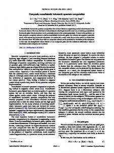
where the selective pulses were applied on the |00i ↔ |01i transition to achieve the exact form of controlled phase gate. The selective excitation was obtained with Gaussian shaped pulses of 13.2 ms duration. The non-adiabatic geometric phase was observed in the phase of |00i ↔ |10i coherence. We have observed the geometric phase for the slice circuit with various solid angles (2φ), each time varying the phase φ of the second selective (π)-pulse. The corresponding spectra are given in figure 2(c), where the |00i ↔ |10i shows a phase change of eiφ . For φ = 0, there is no phase change and the peak is absorptive. With increase of φ, the phase of the peak changes and it becomes dispersive for φ = π/2, and subsequently, a negative absorptive for φ = π. The three small lines in the spectra comes from the naturally abundant 13 C signal of CDCl3 , which provide a reference. Since all dynamical phases due to evolution under chemical shift and J-couplings were refocused, the solvent
13
C signal is absorptive in all the spectra. However, solute
13
C signal
gains phase because it is coupled to the protons, one of whose transition is taken through a closed circuit. This result thus provides a graphic display of geometric phase by non-adiabatic evolution.
To accurately read the phase angle of each spectrum in Fig. 2(c), a zero-order phase correction was applied to the spectra in Fig. 2(c), till the observed peak became absorptive. The change of phase of |00i ↔ |10i coherence due to geometric phase is plotted against the solid-angle (2φ), in figure 3. The graph in figure 3 shows the high fidelity of the experimental implementation of the slice circuit in this case. B. Geometric phase acquired by a triangular circuit
In the triangular circuit, the state vector traverses a triangular path on the Bloch sphere figure 1(c) [18]. The solid angle enclosed by the triangular circuit of figure 1(c) is φ. The controlled phase shift gate can be implemented by the non-adiabatic phase acquired when the appropriate sub-system goes through this circuit. The pulse sequence for the circuit and the corresponding operator can be calculated, similar to that of the sliced circuit, as |10i↔|11i
A.C.B = (π/2)θ 1 0 =
0 0
0
1
0
0
0
0
0
√1 2 sinθ−icosθ
−sinθ−icosθ √ 2 1 √ 2
√1 2
0 × 0
0
1
0
0
0
√1 2 −sin(θ−φ)+icos(θ−φ) √ 2
0 0
1
0
0
0
0
0 e−iφ/2
0 0
0
0 eiφ/2
0 e−iφ/2
0 0
0
0 0 1 0
=
0
1
0 0 1 0
0 0
|10i↔|11i
.(φ)|10i↔|11i .(π/2)θ+π−φ z 1 0 0 0
sin(θ−φ)+icos(θ−φ) √ 2 √1 2
,
0
×
0
eiφ/2
(5)
The intermediate (φ)|10i↔|11i pulse can be applied by the composite z-pulse sequence z |10i↔|11i
(π/2)y|10i↔|11i (φ)−x
|10i↔|11i
(π/2)−y
[33,34].
In the experiments, we have chosen θ = 3π/2. The state of |00i + |10i was prepared and then the pulse sequence of figure 1(d) was applied. Similar to the slice circuit, the sequence was incorporated in a Hahn-echo and the pulses were applied on the |00i ↔ |01i transition. The operator of Eq.[5]
transforms |00i + |10i to |00i + e−iφ/2 |10i. The phase of the |00i ↔ |10i was observed for various φ, by changing the angle of the z-pulse and the phase of the last pulse in Eq.[5]. The spectra are
given in figure 4. Once again, the peak changes from absorptive to dispersive and then to a negative absorptive in correspondence with the change of φ. However, there are two major differences between the spectra of figure 2(c) and 4(c). Note that after the phase gate, the state of the system is |00i + eiφ |10i for slice circuit and |00i + e−iφ/2 |10i for triangular circuit. This is because the solid angle of the slice circuit if 2φ, whereas that of the triangular circuit is φ. Hence, in the slice circuit the coherences become a negative absorptive for φ = π, whereas in the triangle circuit the same observation is obtained for φ = 2π. Moreover, the phase of the pulses corresponding to the triangle circuit is chosen such that the sign of phase is opposite to that of the slice circuit. This difference is clearly reflected in the sign of the coherences between figure 2(c) and 4(c). A plot of the absolute value of observed phase change against solid angle is given in figure 5, whose high fidelity validate the use of such gates for quantum computing. III. DEUTSCH-JOZSA ALGORITHM
Deutsch-Jozsa (DJ) algorithm provides a demonstration of the advantage of quantum superpositions over classical computing [20]. The DJ algorithm determines the type of an unknown function when it is either constant or balanced. In the simplest case, f (x) maps a single bit to a single bit. The function is called constant if f (x) is independent of x and it is balanced if f (x) is zero for one value of x and unity for the other value. For N qubit system, f (x1 , x2 , ...xN ) is constant if it is independent of xi and balanced if it is zero for half the values of xi and unity for the other half. Classically it requires (2N −1 + 1) function calls to check if f (x1 , x2 , ...xN ) is constant or balanced. However the DJ algorithm would require only a single function call [20]. The Cleve version of DJ algorithm implemented by using a unitary transformation by the propagator Uf while adding an extra qubit, is given by [35], Uf
|x1 , x2 , ...xN i|xN +1 i −→ |x1 , x2 , ...xN i|xN +1 ⊕ f (x1 , x2 , ...xN )i
(6)
The four possible functions for the single-bit DJ algorithm are f00 , f11 , f10 and f01 . f00 (x) = 0 for x =0 or 1, f11 (x) = 1 for x =0 or 1, f10 (x) =1 or 0 corresponding to x =0 or 1, while f01 (x) =0 or 1 corresponding to x =0 or 1. The unitary transformations corresponding to the four possible propagators Uf are
Uf00 =
1 0 0 0
0 0
1 0 0 0 1
, 0
Uf11 =
0 0 0 1
Uf10 =
1 0 0 0
0 0
0 1 0 0
1 0
0 0 0 0 0
, 1
0 0 1 0
1 0 0
Uf01 =
,
0 0 1 0 0 1 0
0 1 0 0
1 0
0 0 0
.
0 1 0 0 0 0 1
(7)
For higher qubits the functions are easy to evaluate using Eq.[6]. DJ-algorithm has been demonstrated using dynamic phase by several research groups [29,36–39]. The quantum circuit for single-bit Cleve version of DJ algorithm is given in figure 6(a) [36]. The algorithm starts with |00i pseudopure state. The pair of pseudo-Hadamard gates (π/2)1y (π/2)2−y √ √ create superposition of the form [(|0i + |1i)/ 2][(|0i − |1i)/ 2]. Then the operator Uf is applied. √ When the function is constant, i.e. f (0) = f (1), the input qubit is in the state (|0i + |1i)/ 2, else √ the function is balanced in which case it is in the state (|0i − |1i)/ 2. Thus, the answer is stored in the relative phase between the two states of the input qubit. A final pair of pseudo-Hadamard gates (π/2)1−y (π/2)2y converts the superposition back into the eigenstates. The work qubit comes back to state |0i, where as the input qubit becomes |0i or |1i corresponding to the function being constant or balanced. The operator of Uf00 is identity matrix and corresponds to no operation. The operator of Uf11 can be achieved by a (π)x pulse on the second qubit. In this experiment, unlike section II, we label proton as the first qubit and carbon as the second qubit, and consequently the (π)x pulse was applied on the carbon. The Uf10 operator is a controlled-NOT gate which flips the second qubit when the first qubit is |1i. This gate can be achieved by a controlled phase gate sandwiched between two
pseudo-Hadamard gates on the second qubit [], Uf10 = h − C11 (π) − h−1 , where the controlled phase gate is of the form,
C11 (φ) =
1 0 0
0 0
1 0 0 1
0
0 0
.
(8)
0 0 0 eiφ This precise form of controlled phase gate can be achieved by a recursive use of the phase gates demonstrated in section II. Since the gate A.B given in Eq.[1] attributes a phase eiφ to the state |10i and e−iφ to the state |11i, we denote this gate as C10 (φ).C11 (−φ), where
A.B = [C10 (φ).C11 (−φ)] =
1 0
0 0
1
0
0
0
0
iφ
0 e
0 0
0
e−iφ
0
.
(9)
The phase gate C11 (φ) can be constructed by a suitable combination of these gates, [C00 (−φ/4).C10 (φ/4)] × [C01 (−φ/4).C11 (φ/4)] × [C10 (−φ/2).C11 (φ/2)] −iφ/4 1 0 0 1 0 0 0 e 0 0 0 =
=
0 × 0 0
e−iφ/4
0
0
1
0
1 0
0 0 0
e−iφ/4
0
0
0
1
0
0 eiφ/4
0
0
−iφ/4
e
0
0
0
0
0
0
0
0
−iφ/4
e
0
0 ei3φ/4
=
0 × 0
1
1 0
0 0
0
0 1
0
0 0 0 eiφ
0
0 e−iφ/2
0
0
0 0 0 eiφ/4 1 0 0 0
0 e−iφ/4 0
0
0
eiφ/2
= e−iφ/4 C11 (φ).
(10)
Note that if performed in fault-tolerant manner by using non-adiabatic geometric phase, the first gate requires a rotation of the transition |00i ↔ |10i through a closed circuit. We have used the slice |00i↔|10i
circuit, where it requires a sequence of two π-pulses, (π)θ
|00i↔|10i
(π)θ+π−φ/4 . Similarly, the second
|01i↔|11i
phase gate of Eq.[7] can be achieved by the pulse sequence (π)θ
|01i↔|11i
(π)θ+π−φ/4 . Note that these
two sequence is require pulsing of both the transitions of first qubit, |00i ↔ |10i for the first gate and |01i ↔ |11i for the second. Hence, they can be performed simultaneously by a couple spin-selective
pulses (π)1θ (π)1θ+π−φ/4 , where the pulses are applied on the first qubit (denoted by superscript). Thus, |10i↔|11i
C11 (φ) = (π)1θ .(π)1θ+π−φ/4 .(π)θ
|10i↔|11i
.(π)θ+π−φ/2 .
(11)
In this case φ = π, and we have chosen θ = 3π/2. The last two pulses are however transition selective pulses, which were incorporated into a refocusing sequence, τ − (π/2)1x − τ − (π/2)2x − τ − (π/2)1x − τ − (π/2)2x , where the selective pulses were applied in the last τ period, and the pulses were applied
on the |00i ↔ |01i transition. It may be noted that the triangular circuit could have also used for
the same purpose. The pseudo-Hadamard pulses on second qubit were achieved by h = (π/2)2y and h−1 = (π/2)2−y pulses. The operator of Uf01 can be implemented in the similar manner by h − C00 (π) − h−1 , where C00 (φ) can be implemented by |10i↔|11i
C00 (φ) = (π)1θ .(π)1θ+π+φ/4 .(π)θ
|00i↔|01i
.(π)θ+π+φ/2 .
(12)
The equilibrium spectrum of the two qubits are given in figure 6(b). After creating the superposition from pps, applying the various Uf , and applying the last set of (π/2) pulses, the spectra of proton and carbon were recorded in two different experiments by selective (π/2) pulses after a gradient. The spectra corresponding to various functions are given in figure 6(c), (e), (g) and (i). The intensities of the peaks in the spectra provide a measure of the diagonal elements of the density matrix. The complete tomographed [40,41] density matrices in each case is given in figures 6(d), (f), (h) and (j). When Uf00 and Uf11 are implemented, the final state is |00i, and since the state of input qubit is |0i, the corresponding functions f00 and f11 are inferred to be constant. Whereas in the case of Uf01 and Uf10 , the final state of the system in |10i. The state of input qubit being |1i, the corresponding functions f01 and f10 are balanced. Theoretically, it is expected that the density matrices will have only the populations corresponding to the final pure states. There were however errors due to r.f. inhomogeneity and relaxation. The deviation from the expected results are within 13%. IV. GROVER’S SEARCH ALGORITHM
√ Grover’s search algorithm can search an unsorted database of size N in O( N ) steps while a classical search would require O(N) steps [21]. Grover’s search algorithm has been earlier demonstrated by several workers by NMR, all using dynamic phase [30,42–44,39]. The quantum circuit for implementing Grover’s search algorithm on two qubit system is given in figure 7(a). The algorithm starts from a |00i pseudopure state. A uniform superposition of all states are created by the initial Hadamard gates (H). Then the sign of the searched state “x” is inverted by the oracle through the operator Ux = I − 2|xihx|,
(13)
where Ux is a controlled phase shift gate Cx (π). C11 (π) and C00 (π) gates were implemented by the pulse sequences given in Eq.[11] and [12] respectively. The oracle for the other two states |01i and |10i were implemented by the sequences, |10i↔|11i
.(π)θ+π−φ/2 ,
|10i↔|11i
.(π)θ+π+φ/2 ,
C01 (φ) = (π)1θ .(π)1θ+π+φ/4 .(π)θ C10 (φ) = (π)1θ .(π)1θ+π−φ/4 .(π)θ
|00i↔|01i
|10i↔|11i
(14)
where φ = π, as required in our case. An inversion about mean is performed on all the states by a diffusion operator HU00 H [21], where U00 = I − 2|00ih00|,
(15)
where U00 is nothing but C00 (π), and was implemented by the pulse sequence of Eq.[12]. For an √ N-sized database the algorithm requires O( N ) iterations of Ux HU00 H [21]. For a 2-qubit system with four states, only one iteration is required [30,42]. We have created a |00i pseudopure state using Eq.[3] and applied the quantum circuit of figure 7(a), for |xi = |00i, |01i, |10i and |11i. Finally, the spectra of proton and carbon were recorded individually in two different experiments by selective (π/2) pulses after a gradient. The complete tomographed density matrices in each case is given in figures 7(d), (f), (h) and (j). In each case, the searched state |xi was found to be with highest probability. Ideally in a two-qubit system, probability should exist only in the searched state, and there should be no coherences. Experimentally however, other states were also found with low probability, and some coherences were found in the off-diagonal elements of the density matrix. These errors are mainly due to relaxation and imperfection of pulses caused by r.f. inhomogeneity. Imperfection of r.f. pulses can cause imperfect refocusing of dynamic phase. However, it was found that setting the duration of selective pulses to multiples of (2/J) yielded better results. We have used 13.2ms (6/J) duration Gaussian shaped pulses. The maximum errors in the diagonal elements are within 10% and that in the off-diagonal elemenst are within 15%. V. CONCLUSION
A technique of using non-adiabatic geometric phase for quantum computing by NMR is demonstrated. The technique uses selective excitation of subsystems, and is easily scalable to higher qubit systems provided the spectrum is well resolved. Since the non-adiabatic geometric phase does not depend on the details of the path traversed, it is insusceptible to certain errors yielding inherently fault-tolerant quantum computation [45,46]. The controlled geometric phase gates were also used to implement DJ-algorithm and Grover’s search algorithm in a two-qubit system. Implementation of fault-tolerant controlled phase gates using adiabatic geometric phase demands that the evolution should be ’adiabatic’, which requires long experimental time. To avoid decoherence, use of non-adiabatic geometric phase might be utile. VI. ACKNOWLEDGMENT
The authors thank K.V. Ramanathan for useful discussions. The use of DRX-500 NMR spectrometer funded by the Department of Science and Technology (DST), New Delhi, at the Sophisticated Instruments Facility, Indian Institute of Science, Bangalore, is gratefully acknowledged. AK ac-
knowledges “DAE-BRNS” for senior scientist support and DST for a research grant for ”Quantum Computing by NMR”. ∗
DAE/BRNS Senior Scientist, e-mail:
[email protected]
[1] M.V.Berry, J. Mod. Optics. 34, 1401 (1987). [2] B.Simon, Phys. Rev. Lett. 51, 2167 (1987). [3] Aharonov Y and Anandan J 1987 Phys. Rev. Lett. 58, 1593 (1987). [4] R.P. Feynman, Int J. Theor. Phys. 21, (1982) 467. [5] J.
Preskill,
Lecture
notes
for
Physics
229:
Quantum
information
and
Computation,
http://theory.caltech.edu/people/preskill/. [6] D. Bouwmeester, A. Ekert and A. Zeilinger, (Ed) The Physics of Quantum Information, Springer, 2000. [7] M.A. Nielsen and I.L. Chuang, Quantum Computation and Quantum Information, Cambridge University Press 2000. [8] D.G. Cory, A.F. Fahmy, and T.F. Havel, Proc Natl Acad Sci. USA 94, (1997) 1634. [9] D. G. Cory, M. D. Price and T.F. Havel, Physica D, 120, 82 (1998). [10] N.A. Gershenfeld and I.L. Chuang, Science. 275, (1997) 350. [11] Z.L. Madi, R. Bruschweiler and R.R. Ernst, J. Chem. Phys. 109, 10603. [12] J.A. Jones, Prog. Nucl. Mag. Res. Spec. 38, (2001) 325. [13] J.A. Jones, v. Vedral, A. Ekert and G. Castagnoli Nature 403 869,(2000). [14] A. Ekert, M. Ericsson, P. Hayden, H. Inamori, J.A. Jones, D.K.L. Oi, V.Vedral Journal of Modern Optics 47, 2501 (2000). [15] X.B. Wang and M. Keiji, Phys. Rev. Lett. 87, 097901(2001). [16] S.L. Zhu, Z.D. Wang, Phys. Rev. Lett. 89,97902 (2002) [17] D. Suter, G. Chingas, R. A. Harris and A. Pines, Mol. Phys. 61, 1327 (1987). [18] D. Suter, K.T. Mueller and A. Pines, Phys. Rev. Lett. 60, 1218 (1988). [19] J. Du, P. Zou, M. Shi, L. C. Kwek, Jian-Wei Pan, C. H. Oh, A. Ekert, D. K. L. Oi, and M. Ericsson, Phys. Rev. Lett. 91, 100403 (2003). [20] D. Deutsch and R. Jozsa, Proc. R. Soc. London A 439, (1992) 553. [21] L.K. Grover, Phys. Rev. Lett. 79, (1997) 325.
[22] A. Carollo, I. Fuentes-Guridi, M. Franca Santos, V. Vedral, Phys. Rev. Lett. 90,(2003) 160402. [23] R. Freeman, Spin Choreography, Specktrum (Oxford) 1997. [24] N. Linden, H. Barjat, and R. Freeman Chem. Phys. Lett. 296, 61 (1998). [25] Kavita Dorai, Arvind, Anil Kumar, Phys Rev A. 61, (2000) 042306. [26] Anil Kumar, K. V. Ramanathan, T. S. Mahesh, N. Sinha and K.V.R.M. Murali, Pramana 59 243 (2002). [27] Ranabir Das and Anil Kumar, Phys. Rev. A 68, 032304 (2003). [28] S. Vega, J. Chem. Phys. 68, 5518 (1978). [29] J. A. Jones and M. Mosca, J. Chem. Phys. 109, 1648 (1998). [30] J. A. Jones, M. Mosca and R. H. Hansen, Nature 393 344 (1998). [31] E. L. Hahn, Phys. Rev. 80, 580 (1950). [32] R.R. Ernst, G. Bodenhausen, and A. Wokaun, Principles of Nuclear Magnetic Resonance in One and Two Dimensions, Clarendon Press, Oxford, U.K. 1987. [33] R. Freeman, T.A. Frenkiel and M.H. Levitt, J. Mag. Res.44, 409(1981). [34] Ranabir Das, T.S. Mahesh, and Anil Kumar, J. Magn. Reson. 159 46 (2002). [35] R.Cleve, A. Ekert, C. Macchiavello, and M. Mosca, Proc. Roy. Soc. Lond. A 454, 339 (1998). [36] I. L.Chuang, L. M. K. Vanderspyen, X. Zhou, D.W. Leung, and S. Llyod, Nature (London) 393, 1443 (1998). [37] Kavita Dorai, T. S. Mahesh, Arvind and Anil Kumar, Current Science, 79 (10) 1447 (2000). [38] Arvind, K. Dorai and Anil Kumar, Pramana 56 7705 (2001). [39] Ranabir Das and Anil Kumar, J. Chem. Phys. (in press). [40] I.L. Chuang, N. Greshenfeld, M.Kubinec, and D. Leung, Proc. R. Soc. Lond. A 454, 447 (1998). [41] Ranabir Das, T.S. Mahesh, and Anil Kumar, Phys. Rev. A. 67, 062304 (2003). [42] I. L. Chuang, N. Gershenfeld, and M. Kubinec, Phys. Rev. Lett. 80, 3408-3411 (1998). [43] L.M.K. Vanderspypen, M. Steffen, M.H. Sherwood, C.S. Yannoni,R. Cleve, and I.L. Chuang, Applied Physics Lett. 76, (2000) 646. [44] Ranabir Das, T.S. Mahesh, and Anil Kumar, Chem. Phys. Lett. 369, 8 (2003). [45] A. Y. Kitaev, quant-ph/9707021. [46] J. Preskill, quant-ph/9712048.
Figure captions Figure 1: (a) The transport of a selected subsystem of two states |ri and |si through slice circuit [18]. (b) Corresponding pulse sequence. A and B are transition selective pulses incorporated into a |ri↔|si
Hahn-echo [18], where A= (π)θ
|ri↔|si
and B= (π)θ+π+φ . The path of the polarization vector under |ri↔|si
applied r.f. pulses is shown as A and B in (a). Due to the A= (π)θ
pulse, the polarization
traverses a path from +z to -z. It comes back to +z along a different path if it is rotated about an axis with azimuthal angle (θ + π + φ), therby enclosing a sliced circuit of solid angle 2φ. (c) The transport of a selected subsystem of two states |ri and |si through a triangular circuit [18]. (d) Pulse |ri↔|si
sequence for implementation of the triangular circuit given in (c). A=(π/2)θ |ri↔|si
|ri↔|si
B= (π/2)θ+π−φ . The polarization vector is flipped to xy-plane by (π/2)θ
, C= (φ)|ri↔|si and z
, rotated about z-axis
and brought back to the z-axis by a (π/2)|ri↔|si rotation about (θ + π − φ). The solid by (φ)|ri↔|si z angle enclosed by the circuit is φ.
Figure 2: Observation of non-adiabatic geometric phase when the subsystem is taken through the slice circuit of figure 1(a). (a) Equilibrium the natural abundant
13
13
C spectrum of 13 CHCl3 . The three small lines are from
C signal from the solvent of CDCl3 . (b) The
13
C coherence of the prepared
|00i + |10i state. (c) The 13 C coherence of the state |00i + eiφ |10i. Since the subsystem goes through a closed circuit, the coherence gains a phase of purely geometric origin, the magnitude of which is proportional to the solid angle (2φ) of the circuit. It may be noted that since all dynamical phases are refocused, the solvent signal from CDCl3 is always absorptive irrespective of φ. The solute (13 CHCl3 ) signal on the other hand gains a phase of φ. The resulting signal changes shape from pure absorptive for φ = 0, to intermediate phase for arbitrary φ, dispersive for φ = π/2 and to absorptive (negative sign) for φ = π.
Figure 3: The geometric phase gained by the
13
C coherence in Fig 2(c) is plotted against the
corresponding solid angle (2φ). The observed phase closely matches the expected.
Figure 4: Observation of non-adiabatic geometric phase when the subsystem is taken through the triangular circuit of figure 1(c). (a) Equilibrium of the prepared |00i + |10i state. (c) The
13
13
C spectrum of
13
CHCl3 . (b) The
13
C coherence
C coherence of the state |00i + e−iφ/2 |10i, after the
subsystem goes through the triangular closed circuit. The coherence changes from absorptive to dispersive and then to a negative absorptive with the change of φ. It may be noted that sign of
phase of the coherence is opposite to that of 2(c).
Figure 5: A plot of the absolute value of observed geometric phase gained by the
13
C coherence in
Fig 4(c) is plotted against the corresponding solid angle (φ). The plot demonstrates high fidelity of such gates. Figure 6: Implementation of DJ-algorithm using non-adiabatic geometric phase in the two-qubit system of
13
CHCl3 . (a) Quantum circuit for implementation of DJ-algorithm in a two-qubit system
[36]. h=(π/2)y and h−1 =(π/2)−y (b) Equilibrium 1 H and
13
C spectra. (c) The 1 H and
13
C spectra
obtained after completion of the quantum circuit of (a) for Uf00 , and application of a gradient pulse followed by (π/2) pulses on 1 H and
13
C individually. (d) The complete tomographed density matrix
[40]. The real and imaginary parts of the density matrix are given separately with the imaginary part being magnified five times (×5). (e), (g) and (i) are respective spectra obtained after Uf11 , Uf01 and Uf10 . (f), (h) and (j) are the corresponding tomographed density matrices. For constant cases (c) and (e), the final state is |00i, as shown in (d) and (f). For balanced cases (g) and (i), the final state in |10i, as shown in (h) and (i). The diagonal elements have a fidelity of 95%, while off-diagonal parts have a fidelity of 87%.
Figure 7: Implementation of Grover’s search algorithm using non-adiabatic geometric phase in the two-qubit system of
13
CHCl3 . (a) Quantum circuit for implementation of Grover’s search algorithm
in a two-qubit system [42,30]. The Ux and U00 phase gates were implemented by non-adiabatic geometric phase using selective excitation by 13.2 ms (6/J) long Gaussian shaped pulses. (b) Equilibrium 1 H and
13
C spectra. (c) The 1 H and
13
C spectra obtained after completion of the quantum
circuit of (a) for |xi = |00i, and application of a gradient pulse followed by (π/2) pulses on 1 H and
13
C individually. The intensities of the various lines in the spectrum gives the populations of
the density matrix. (d) The complete tomographed density matrix [40] after implementation of the quantum circuit (a) for x = |00i. The real and imaginary parts of the density matrix are given separately and the imaginary part is magnified five times (×5). (e), (g) and (i) are the spectra obtained when |xi = |01i, |xi = |10i and |xi = |11i. In each case the searched state |xi was found with highest probability after implementation of the search algorithm with a fidelity more than 85%.
(a)
(θ+π+φ)
(b)
z B
A
|0 + |1
θ
φ
(π) x
(π)−x
τ
τ
φ
Figure 1
(θ+π)
A
B
|0
(θ+π/2)
(c)
B
A (θ+π) (θ+π−φ) (θ+π/2)
(d)
z
φ φ
|0 + |1
(π) x
(π)−x
τ
τ
θ
C |0
A
C
B
(b)|00 +|10
(a)Equ 13
C
100
0
−100
Hz
100
(c)|00 + e
iφ
0
|10
φ=0
φ=π/8
φ=2π/8
φ=3π/8
φ=4π/8
φ=5π/8
φ=6π/8
φ=7π/8
φ=π
Figure 2
−100
Hz
π
Geometric phase (observed)
7π/8 6π/8 5π/8 4π/8 3π/8 2π/8 π/8 0
0
π/4
2π/4
3π/4 4π/4 5π/4 Solid angle
Figure 3
6π/4
7π/4
2π
(b)|00 +|10
(a)Equ 13
C
100
0
−100
Hz
100
0
−i φ/2
(c)|00 +e
|10
φ=0
φ=π/4
φ=2π/4
φ=3π/4
φ=4π/4
φ=5π/4
φ=6π/4
φ=7π/4
φ=2π
Figure 4
−100
Hz
π
Geometric phase (observed)
7π/8 6π/8 5π/8 4π/8 3π/8 2π/8 π/8 0
0
π/4
2π/4
3π/4 4π/4 5π/4 Solid angle
Figure 5
6π/4
7π/4
2π
(a)
+1 0−
0 +1 h
0
h−1
0
1
(b)
100
(c)
13
H
0
Hz
100
0−1
Uf
0+1
h−1
0
h
0
0
Hz
(d)
REAL
IMAGINARY X 5
1
0.2
0.5
0
0 00 01 10 11
(e)
0
Hz
100
0
Hz
00 01
10 11
−0.2 00 01 10 11
00 01
10 11
(f) X 5
f11
1
0.2
0.5
0
0 00 01 10 11
100
1
C
f00
100
or
0
Hz
100
0
00 01
10 11
−0.2 00 01 10 11
00 01
10 11
Hz
(h) X 5 1
(g)
0.5
f01
0
0 00 01 10 11
100
0.2
0
Hz
100
0
00 01
10 11
−0.2 00 01 10 11
f10
X 5
1
0.2
0.5
0
0 00 01 10 11
100
0
Hz
100
0
10 11
Hz
(j)
(i)
00 01
Hz
Figure 6
00 01
10 11
−0.2 00 01 10 11
00 01
10 11
(a) H
0
H
H
U00
Ux H
0
(b)
100
1
13
H
0
Hz
100
H
H
C
0
Hz
(d)
IMAGINARY
REAL
X 5
(c)
1
0.2
0.5
0
0 00 01 10 11
100
0
Hz
100
0
00 01
10 11
−0.2 00 01 10 11
(e)
X 5
1
0.2
0.5
0
0 00 01 10 11
0
Hz
100
0
00 01
10 11
−0.2 00 01 10 11
(g)
0.2
0.5
0
00 01 10 11
Hz
100
0
00 01
10 11
−0.2 00 01 10 11
(i)
0.2
0.5
0
00 01 10 11
Hz
100
0
10 11
X 5
1
0
0
00 01
Hz
(j)
100
10 11
X 5
1
0
0
00 01
Hz
(h)
100
10 11
Hz
(f)
100
00 01
Hz
Figure 7
00 01
10 11
−0.2 00 01 10 11
00 01
10 11