Game playing usually uses Artificial intelligence as its prime domain. Two player games do not fit into the established RL framework as the optimality criterion for ...
International Journal of Computer Applications (0975 – 8887) Volume 69– No.22, May 2013
Use of Reinforcement Learning as a Challenge: A Review Rashmi Sharma
Manish Prateek
Ashok K. Sinha
Research Scholar Department of Computer Science UPES, Dehradun
Professor & Head Department of Computer Science UPES, Dehradun
Professor & Head Department of Information Technology ABES Engg College, Gzd
ABSTRACT Reinforcement learning has its origin from the animal learning theory. RL does not require prior knowledge but can autonomously get optional policy with the help of knowledge obtained by trial-and-error and continuously interacting with the dynamic environment. Due to its characteristics of self improving and online learning, reinforcement learning has become one of intelligent agent’s core technologies. This paper gives an introduction of reinforcement learning, discusses its basic model, the optimal policies used in RL , the main reinforcement optimal policy that are used to reward the agent including model free and model based policies – Temporal difference method, Q-learning , average reward, certainty equivalent methods, Dyna , prioritized sweeping , queue Dyna . At last but not the least this paper briefly describe the applications of reinforcement leaning and some of the future research scope in Reinforcement Learning.
General Terms Reinforcement Learning, Q-Learning, temporal difference, robot control.
Keywords Reinforcement Learning, Q-Learning, temporal difference, robot control.
1. INTRODUCTION Reinforcement learning (RL) or self learning technology has its origin from some subjects: statistics, control theory and psychology and so on. It has a very long history, until the late 80s and early 90s that reinforcement learning technology obtains the wide research and application in some fields such as artificial intelligence(AI), machine learning, automatic control and so on [1] . RL is one of the techniques in artificial intelligence (AI) which is usually considered as a goaldirected method for solving problems in uncertain and dynamic environments. RL refers to a category of unsupervised machine learning algorithms that seek to maximize a reward signal. Supervised learning methods utilizes examples of correct action, but RL methods learns by trying many actions and learns which of those actions produce the most reward. Reinforcement learning is an important machine learning method [2], its learning technology can be of three different types: 1. Supervised learning, 2. Unsupervised learning and 3. Reinforcement learning. RL is an online learning technology which is quite different from supervised learning and unsupervised learning. RL differs from the supervised learning (SL) in following aspects: In SL an agent learns from examples which are provided by a knowledgeable external supervisor, In RL the
agent learn by directly interacting with the system and its environment and after choosing an action the agent is immediately communicated the reward or punishment and the subsequent state .The evaluation of the system is in concurrent to the learning. In RL no input/output pairs are presented, in SL expected future predictive accuracy or statistical efficiency is the prime concerns.
1.1
Basic Model of RL
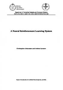
A RL model consists of a. A discrete set of environment states S b. A discrete set of agent action A c. A set of scalar reinforcement signals {0, 1} or the real numbers. A reinforcement learning agent is autonomous [3] which means that its behavior is determined by its own experience. Learning is the mechanism through which an agent can increase its intelligence while performing operations. What is outside the agent is considered the environment. The states are parameters or features that describe the environment. An RL agent senses the environment and learns the optimal policy or near optimal policy by taking actions in each state of the environment. The agent must be aware of the states while interacting with the environment. An agent learns from reinforcement feedback received from its environment known as either reward or punishment signal. RL agents try to maximize the reward or minimize the punishment [4, 5, 6]. Actions could affect the next state of the environment and subsequent rewards and have the ability to optimize the environment’s state [7]. Continuous learning and adapting through interaction with environment helps the agent to learn online in terms of performing the required task and improving its behavior in real time. Figure 1 shows the basic model of the reinforcement signal. Stepwise execution of basic model of RL 1. Intelligent agent receives as input ‘i’ , some indication of current state (s1) of the environment 2. The intelligent agent then chooses an action from the set of actions (A) to generate as output 3. (a) The action changes the state of environment (s2) (b) The value of this state transition is communicated to the agent through a scalar reinforcement signal (r) One of the significant issues is how to improve an autonomous agent’s capability and how to enhance the agent’s intelligence. The ability of an agent can increase its intelligence through learning while in operation. Knowledge gained by an RL agent is specific to the environment in which it operates and cannot be easily transferred to another agent, even if the environments are very similar. The general
28
International Journal of Computer Applications (0975 – 8887) Volume 69– No.22, May 2013 knowledge obtained from one agent could benefit the other, but no efficient methods exist for transfer of that knowledge.
State
γ can be interpreted as an interest rate , a probability of executing another step or a mathematical trick to bound the infinite sum . The discounted model is more tractable as compared to finite-horizon model and resembles recedinghorizon model so widely used model.
S1 3(b) Intelligent Agent
Environment
In the average-reward model the agent takes actions which optimize its long-run average rewards. This policy is also known as gain optimal policy. This is the limiting case of the discounted model when its factor approaches value 1.
2 (3) Action
3(a) The model can be generalized so that it takes into account the long run average and the amount gained by the initial reward.
Figure1. A Basic Model of RL An RL agent’s design is based on the characteristics of the problem to be solved. The problem must be clearly defined and analyzed so that the purpose of designing the agent can be determined. The RL agent is a decision-maker in the process which takes an action that influences the environment. The agent acquires knowledge of different actions and eventually learns to perform actions which are most rewarding in order to attain a certain goal. Another key element of RL is an action policy which defines the agent’s behavior at any given time and it maps the states to the actions to be taken [6].
1.2 Optimal Policies of RL Before thinking about learning algorithms to behave optimally, decision about the models of optimality should be done. In particular, the behavior of an agent now decides how the agent will behave in future. So, the decisions made depend on the reward or the punishment signals generated as a result of transition of state of the environment. There are four optimality criterions used for generation of scalar reward/punishment signal: Finite- horizon model, recedinghorizon control, infinite-horizon discounted model, and average-reward model [7]. The finite-horizon model is the easiest model. In this model, at a given moment the agent should optimize its expected reward for the next n steps: E( (1) In the expressions ri represents the scalar reward after n steps into the future. This model has a drawback that precise length of the agent’s life cannot be known in advance and so this model is always inappropriate. The receding-horizon policy always takes n-step optimal action. The agent acts always according to the same policy, the value of n limits how far an agent looks in choosing its actions. The infinite-horizon discounted model takes into account a long-run reward of the agent. The rewards received in the future are geometrically discounted according to the discounted factor γ whose value should lie between 0 and 1 E(
(2)
In general, bias optimality model, a policy is preferred if it maximizes the long-run average and the ties are broken by the initial extra reward. The choice of optimality model and the choice of parameters matters much and so should be chosen carefully.
1.3 Challenges in Reinforcement Learning The system developed using RL or self learning requires being intelligent enough to take decisions according to the environment changes. The two most commonly and critical applications of self learning (RL) are: robot soccer and mars rover. These require accuracy, agility actions, and flexible strategy. The conditions are dynamic, uncertain and complex and have to take decisions as humans. These systems require general control subsystem, visual subsystem, decision subsystems, communication subsystem and the robot vehicle subsystems. The hardware required is robot vehicle system, the image acquisition device, host computer(s), wireless launchers. These multi-agent system (MAS) uses robotics, artificial intelligence, intelligent control, computer technology, sensor technology. The systems are critical as they have to train themselves for unknown environment about which less or no information is available. Mars rover had objective of investigating mars’ habitability, studying its climate and geology and collecting data for a manned mission to mars. It’s difficult to train the system so that the system developed can fulfil the targeted objective. These system developments require the in-depth study of reinforcement learning or self learning.
2. LEARNING OF OPTIMAL POLICY For a Markov Decision Problems (MDP), to obtain an optimal policy a model is already present. An MDP model is usually consists of a. b. c. d.
A discrete set of environment states S A discrete set of agent action A A reward function R: S Х A →Ŕ A state transition probability function P: S Х A →∏(s), where ∏(s) is probability distributed over the set of environment state S. In other words, it maps different states to its probabilities.
29
International Journal of Computer Applications (0975 – 8887) Volume 69– No.22, May 2013 P(s1,a,s2) denotes probability of state transition from state s1 to state s2 using action a. R(s1,a) denotes immediate reward value obtained when the environment state s1 changes to state s2 using action a. The model is markov, when the state transitions are independent of any previous states or the agent actions. Reinforcement learning is mainly concerned with how an optimal policy can be obtained when a model is not known in advance. The agent directly interacts with the environment to obtain information, which is processed through appropriate algorithm to produce an optimal policy. The two ways in which it can be proceed: Model-free method and model based methods. In model-free method a controller is learnt without learning a model whereas in model-based method [7] first the algorithm is learnt then it is used to derive a controller. Some model-free methods are : temporal difference methods, Qlearning , average rewards and model based methods are : Certainty equivalent , Dyna , queue Dyna , priority sweeping
2.1 Model – Free Methods
Where
=
TEMPORARAL DIFFERENCE METHODS (TD (λ)) The two main components are: a critic and a RL component. The critic uses the real external reinforcement signal to learn to map states with its expected discounted values given that the executing policy is the one currently initiated by the RL component. The experience tuple is usually defined as which summarizes a single transition in the environment. Here s1 is the agent’s state before the transition, a is the choice of action from the set of actions, r is the immediate reward the agent receives and s2 is the resulting state. TD(λ) was proposed by Sutton’s in 1988[8], and combines the Monte Carlo algorithm and the dynamic programming technology. A step of this is TD(0), in which refers to only a step back for the immediate reward value and to modify the estimated value of the resulting state . In TD (0), the update rule used to learn the value of policy is V(s1) = V(s1) +α(r+γ V(s2)- V(s1)) (5) This rule can also be rewritten as V(s1) = (1- α)V(s1) + α(r+γ V(s2)) (6) Whenever a state s1 is visited, its estimated value is updated to be closer to r+γV(s2) , since r is the immediate reward received and V(s2) is the estimated value of the actually occurring next state. If the learning rate α is adjusted properly and the policy is held fixed, TD (0) will guaranteed to converge to the optimal value function. The general TD (λ) rule is similar to TD (0) rule given in equation
1 0
if s = si otherwise
(8)
The eligibility of a state s is the degree, to which it is visited in the recent past. When a reinforcement signal is received, it should update all the states that have been recently visited according to their eligibility criteria. When λ= 0 then it becomes TD(0), when λ=1 , it is roughly equivalent to the updating all the states according to the number of times they are visited till the end of the run .So the eligibility trace is updated as follows : E(s) =
This method shows how it is possible to learn an optimal policy without knowing the models and even without learning those models. Many of these methods described below guarantees to find an optimal policy and use little computation time per experience .They extremely inefficiently use the data they gather and therefore require a great deal of experience to achieve good performance. Temporal credit assignment is the biggest problem faced by RL agent. The decision that the action just taken is a good one or a bad one is difficult as they have far-reaching effects. One solution strategy is to wait till the end and reward the actions taken if the result is good and punish the action if the result is bad. In the current task, it is difficult to know the end and to keep the record of the actions a great deal of memory is required. Second solution is to adjust the estimated value of state based on the immediate reward and the estimated value of the next state. These are called temporal difference (TD (λ)) methods.
V(s1) = V(s1) +α(r+γ V(s2) - V(s1))e(u)
This rule is applied to every state according to its eligibility e(u) rather than just applying to the immediate previous state. The eligibility trace is defined as
if s = current state Otherwise (9)
The execution of TD(λ) is computationally more expensive and converges faster for larger values of λ. Q-LEARNING Q-learning algorithm was proposed by Watkins’ [9, 10] and is easier to implement. Let Q* (s1,a) be the expected discounted reinforcement of taking action a in the state s1, then continues by choosing action optimally . Let V*(s1) = maxa Q*(s1,a) where V*(s1) is the value of s1 with the assumption that the best action is taken initially. The recursion formula of Q* (s1, a) is as follows: Q*(s1,a)=R(s1,a)+γ (s1,a,s2)maxaQ*(s2,a’) (10) The optimal policy would be given by Π*(s) = arg maxa Q*(s1 ,a) (11) The Q function makes the action explicit, so estimate the Q values on-line using a method same as TD (0), but also use them to define the policy. The action can be chosen by taking the one which has the maximum Q value for the current state. The Q-learning rule is given by: Q(s1,a)= Q(s1,a) + α (r + γ maxa Q*(s2 ,a’) - Q(s1,a)) (12) This can be rewritten as Q(s1,a) = (1- α ) Q(s1,a) + α (r + γ maxa Q*(s2 ,a’) ) (13) where < s1,a,r, s2 > is an experiencing tuple. If α decays appropriately and each action is executed in each state an infinite number of times in an infinite run then Q-values will converge with a probability of 1 to Q*. When Q values are nearly converged to their optimal values, the agent can act greedily by selection the actions with the highest Q value. Q-learning is exploration insensitive i.e. the Q values will converge to optimal values, independent of how an agent behaves when the data is being collected. The details of the exploration strategy do not affect the convergence of the learning algorithm. Q-learning is the most popular and most effective model-free algorithm for learning from delayed environment. Q-learning can be applied to discounted infinitehorizon MDPs. Q-learning can also be applied to undiscounted problems if the optimal policy is guaranteed to reach a reward-free state and the state is periodically reset.
(7)
30
International Journal of Computer Applications (0975 – 8887) Volume 69– No.22, May 2013 AVERAGE REWARD (R-LEARNING) Schwartz’s [11] R-learning algorithm exhibits convergence to some of the MDPs. Several researchers have found this average reward criterion closer to the true problems which are being solved by discounted criterion. Mahadevan [12] showed that existing reinforcement learning algorithms for average reward does not always produce bias-optimal policies. Jordon, Singh and Jaakkola [13] described the average reward learning algorithm with guaranteed convergence. It uses monte-carlo component to estimate the expected future rewards for each state as the agent’s moves in the environment.
2.2 Model –Based Methods Assume that the model is not known in advance, examine the algorithms that do operate by learning these models. These algorithms are important in applications in which computation is considered to be cheap and has costly real-world experiences. CERTAINTY EQUIVALENT METHODS In this method, first learn the T and R functions by exploring the environment and keeping statistics about the results of each action then compute an optimal policy using one of the methods of section 2.1. This method is known as Certainty equivalence. The model is learned continually through the agent’s lifetime. At each step the current model is used to compute the value function and an optimal policy. This method makes very effective use of available data but ignores exploration and is extremely computationally demanding for even a small state space. DYNA Sutton’s Dyna Architecture [14, 15] yields strategies that are both more effective than model-free learning and are more computationally efficient than the certainty –equivalence method. It uses experience to build a model, uses experience to adjust the policy and uses model to adjust the policy. Dyna operates in a loop of interaction with the environment. The steps carried out in Dyna algorithm are as follows: 1. Update the model, by incrementing statistics for the transition from state s1 to s2 on action a and for receiving the immediate reward r for taking action a in state s1. The updated models are Ť and Ř. 2. Update the policy at state s1 based on newly updated model using the rule Q(s1,a)= Ř(s1,a)+γ (s1,a,s2) maxa’ Q*(s2 ,a’) (14) This is the value-iteration update for Q values. 3. Perform k additional updates : k state- action pairs are chosen at random and the updation is done accordingly Q(sk,ak)=Ř(sk,ak)+γ (sk,ak,s2)maxa’Q*(s2,a’) (15) 4. Choose an action a’ to perform in state s2 , based on the Q values which is modified by exploration strategy. The algorithm requires about k times the computation of qlearning per instance. A reasonable value of k can be determined based on the relative speeds of computation and of taking action. Dyna requires fewer steps of experience in terms of order of magnitude than Q-learning to arrive at an optimal policy. Dyna requires approximately six times more computational efforts. QUEUE DYNA / PRIORITIZED SWEEPING Dyna suffers from being undirected which means it is unhelpful when the goal has just been reached or the agent has struck in some dead end , it continues to update random state-
action pairs rather than concentrating on the parts of the state space. These problems are solved by Queue-Dyna and Prioritized sweeping which are two independent but very similar techniques. The algorithm is similar to Dyna, except updation are no longer chosen at random and the values are now associated with the states instead of state-action pairs. Some additional information is also stored in the model. Each state keeps an account of its predecessors: the states which have non-zero transition probability under some action. Initially priority of each state is set to zero. Instead of updating k random state-action pairs, prioritized sweeping updates k highest priority states. For each state s with highpriority, it works as follows [7] : 1. The current value of the state Vold = V(s) 2. Update the state’s value as V(s) = maxa (Ř(s,a) +γ∑s’ Ť(s1 , a,s2)V(s2)) (16) 3. Set the state’s priority back to 0. 4. Compute the value change δ =|Vold –V(s)| 5. Use δ to modify the priorities of the predecessor of s. Update the value of V for state s2 and it has changed by amount δ, then immediate predecessors of s2 are informed regarding this event. Any state s1 for which there exists an action a such that Ť(s1,a,s2)≠ 0 then its priority is increased by δ ·Ť(s1 , a,s2) unless its priority has already exceeded that value. The optimal policy is reached in about half the number of steps of experience and one-third the computation as Dyna required. About 20 times fewer steps and twice the computational effort of Q-learning is required by Dyna.
3. STRENGTHS AND LIMITATIONS OF REINFORCEMENT LEARNING 3.1 Strengths a) RL does not require explicit examples of executing correct action b) RL can be applied to systems for which such examples are not readily available. c) RL methods have been used to train neural networks [16], to control dynamic channel assignment in communications networks [17], and to construct fuzzy logic rule bases for fuzzy control systems [18]. d) RL methods find the solution of many diverse problems.
3.2 Limitations a) RL methods tend to learn very slowly, which leads to poor performance in dynamic environments [19]. b) The tradeoffs between exploration and exploitation have to be found. RL agents tries to reach a goal as quickly as possible (exploitation), they also seek to learn more information about their environment in order to enhance the future performance (exploration). c) The exploration/ exploitation dilemma is analogous to the tradeoff between system control and system identification in the field of optimal control [20]. d) Knowledge transfer from one agent to another is another difficulty when considering RL systems [21]. This is due to the fact that RL is a global learning method that contains all of the information learned about the environment in a single value function.
4. APPLICATIONS OF RL RL is a theoretical tool for studying the principles of agents learning to act. RL is also used as a practical computational tool for constructing autonomous systems which improves
31
International Journal of Computer Applications (0975 – 8887) Volume 69– No.22, May 2013 themselves with its own experiences. These applications range from industrial manufacturing, to robotics to combinational search problems used in gaming.[7] Practical applications give a proof for the effectiveness, ability and usefulness of the learning algorithm. This also helps in deciding which components of RL framework are important for practical applications.
4.1
Gaming
Game playing usually uses Artificial intelligence as its prime domain. Two player games do not fit into the established RL framework as the optimality criterion for the games is not of maximizing the rewards but one of the maximizing rewards against an optimal adversary (mini-max). RL algorithms can be adapted to work for a very general class of problems [24], and many researchers have used RL in these environment.
4.2
Robotics and control
There are many applications in robotics and control systems that have used RL. Consider four examples of robotics and one of control system a) A two armed robot [22] was constructed by Schaal and Atkeson which learns to juggle a device known as a devil stick. This complex nonlinear control task involves a 6dimensional state space and less than 200 msecs per control decision. After 40 initial attempts the robot learns to keep jiggling for hundreds of hits. b) A mobile robot pushes large boxes for extended periods of time [23]. Box-pushing is a difficult robotics problem, and characterised by immense uncertainty in the action results. Q-learning along with some novel clustering enables a higher – dimensional input. c) Four mobile robots [7] travelled within an enclosure collecting small disks and transporting to a destination region. In this the three steps were: first pre-programmed signals (progress estimators) were used to break monolithic tasks into subtasks. Second, the control was decentralized. Thirdly, the state space was dividing into smaller number of discrete states according to the values of a small number of pre-programmed Boolean features of the underlying sensors. d) Elevator dispatching task involved four elevator serving ten floors [25] the objective was to minimise the average squared wait time for passengers, discounted into future time. e) Packing tasks from a food processing industry:[7] this problem involves filling containers with erratic numbers of dissimilar products. The product characteristics can be sensed which also vary with time. These examples can be discussed on the following points. f) Robot soccer game is a good platform for the multi agent system (MAS) domain research. In this application proper platform, the research results of artificial intelligence and robotics can be tested and validated, thereby promoting the development of the various fields. The soccer game is a special MAS in that the robot players of one team have to cooperate while facing competition with the opponent. The cooperative and competitive strategies used play a major role in robot soccer system[26] g) A Mars rover is an automated motor vehicle which propels itself across the surface of the planet Mars after landing. Rovers have several advantages over stationary landers: they examine more territory, they can be directed to interesting features, they can place themselves in sunny positions to weather winter months and they can advance
the knowledge of how to perform very remote robotic vehicle control [33].
Pre-programmed knowledge Linearity assumption for the misleading robot's policy[7] , a manual breaking up of the task into subtasks for the two mobile-robot , while the box-pusher also used a clustering technique for the Q values which assumed locally consistent Q values. The four disk-collecting robots used a manually discredited state space. The packaging example had fewer dimensions and so required correspondingly weaker assumptions, but the assumption of local piecewise continuity in the transition model enabled massive reductions in the amount of learning data required.
Exploration strategies The juggler used careful statistical analysis to judge where to profitably experiment. Both mobile robot applications were able to learn well with greedy exploration-always exploiting without intentional exploration. The packaging task used optimism in the face of uncertainty [7].
Computational regimes of the experiment They were all very different, which indicates that the differing computational demands of various RL learning algorithms. The juggler needed to make very fast decisions with low latency between each hit, but had long periods of 30 seconds and more between each trial to consolidate the experiences collected on the previous trial and to perform the computation necessary to produce a new reactive controller on the next trial [22]. The box-pushing robot was meant to operate autonomously for hours and so had to make decisions with a uniform length control cycle. The cycle for substantial computations was sufficiently long. [23]. In the four disk-collecting robots, each robot had a short life of less than 20 minutes, due to battery constraints so the substantial number crushing was impractical, and any significant combinatorial search would have used a significant fraction of the robot's learning lifetime [7]. The packaging task had easy constraints [7]. One decision was needed every few minutes. This provided opportunities for fully computing the optimal value function for the 200,000state system between every control cycle, in addition to performing massive cross-validation-based optimization of the transition model being learned.
5. PRESENT STATUS OF RESEARCH AREA RL is used in almost all the research areas. The researches have been carried out in Job-shop scheduling, Global search algorithm, Behavior arbitration of Robot, Street Car bunching control, Bidding strategic in electricity markets, Operation scheduling in container terminals, intelligent search in unstructured peer –to –peer network, motor skill for wearing T-shirt using topology coordinates, robot learning with Genetic algorithm based fuzzy RL agents, autonomous and fast robot learning through motivation, personalized web document filtering, coordination of communication in robot team, mobile robot navigation , machine learning approaches inn robot navigation , neuromuscular control of the point-topoint and oscillatory movements of saggital arm with the actor, interconnected learning automata, vibration control of a non-linear quater-car active suspension system, acquisition of a page turning skill for a multi-fingered hand, humanoid rhythmic walking parameter based on visual information, 3D
32
International Journal of Computer Applications (0975 – 8887) Volume 69– No.22, May 2013 kinetic Human-Robot cooperation with an EMG to activation model, global supply chain management.
6. CONCLUSION There are a large variety of RL techniques that work effectively on a variety of small problems. But there exist very few techniques that can be scaled to larger problems. The problem is it is very difficult to solve arbitrary problems in the general case. The bias can come in any of the form: shaping, local reinforcement signals, imitation, problem decomposition, reflexes. With appropriate biases, supplied by human programmers or teachers, complex RL problems will eventually be solvable. Many works is still to be carried out and many questions remaining for learning techniques regarding methods for approximation, decomposition and incorporation of bias into real life problems.
7. REFERENCES [1] Singh S, Agents and reinforcement learning [M]. San Matco, CA, USA: Miller freeman publish Inc, 1997. [2] Bush R R & Mosteller F. Stochastic Models for Learning [M]. New York: Wiley, 1955. [3] C. Ribeiro, Reinforcement learning agent, Artificial Intelligence Review 17 (2002) 223–250. [4] A. Ayesh, Emotionally motivated reinforcement learning based controller, in: IEEE SMC, The Hague, The Netherlands, 2004. [5] S. Gadanho, Reinforcement learning in autonomous robots: an empirical investigation of the role of emotions,PhDThesis, University of Edinburgh, Edinburgh, 1999. [6] R.S. Sutton, A.G. Barto, Reinforcement Learning: An Introduction, MIT Press, Cambridge, MA, 1998. [7] L.P. Kaelbling, M.L. Littman, A.W. Moore, Reinforcement learning: a survey, Journal of Artificial Intelligence Research 4 (1996) 237–285. [8] Richard S. Sutton. Learning to predict by the method of temporal differences. Machine Learning, 3(1):9-44, 1988. [9] Christopher J. C. H. Watkins. Learning from Delayed Rewards. PhD thesis, King's College, Cambridge, UK, 1989. [10] Christopher J. C. H. Watkins and Peter Dayan. Qlearning. Machine Learning, 8(3):279-292, 1992. [11] Anton Schwartz. A reinforcement learning method for maximizing undiscounted rewards. In Proceedings of the Tenth International Conference on Machine Learning, pages 298-305, Amherst, Massachusetts, 1993. Morgan Kaufmann. [12] Sridhar Mahadevan. Average reward reinforcement learning: Foundations, algorithms, and empirical results. Machine Learning, 22(1), 1996. [13] Tommi Jaakkola, Satinder Pal Singh, and Michael I. Jordan. Monte-carlo reinforcement learning in nonMarkovian decision problems. In G. Tesauro, D. S. Touretzky, and T. K. Leen, editors, Advances in Neural Information Processing Systems 7, Cambridge, MA, 1995. The MIT Press.
[14] Richard S. Sutton. Integrated architectures for learning, planning, and reacting based on approximating dynamic programming. In Proceedings of the Seventh International Conference on Machine Learning, Austin, TX, 1990. Morgan Kaufmann. [15] Richard S. Sutton. Planning by incremental dynamic programming. In Proceedings of the Eighth International Workshop on Machine Learning, pages 353-357. Morgan Kaufmann,1991. [16] Tesauro, G. J., Temporal difference learning and TDGammon.Commun. ACM 38, 58–68 (1995). [17] Nie, J. and Haykin, S., A dynamic channel assignment policy through Q-learning. IEEE Trans. Neural Netw.10, 1443–1455 (1999). [18] Beom, H. R. and Cho, H. S., A sensor-based navigation for a mobile robot using fuzzy logic and reinforcement learning. IEEE Trans. Syst. Man Cybern. 25, 464–477 (1995). [19] Coelho, J. A., Araujo, E. G., Huber, M., and Grupen, R. A., Dynamical categories and control policy selection.Proceedings of IEEE International Symposium on Intelligent Control, 1998, pp. 459–464. [20] Witten, I. H., The apparent conflict between estimation and control—A survey of the two-armed problem. J. Franklin Inst. 301, 161–189 (1976) [21] Malak, R. J. and Khosla, P. K., A framework for the adaptive transfer of robot skill knowledge using reinforcement learning agents. Proceedings of IEEE International Conference on Robotics and Automation, 2001, pp. 1994–2001. [22] S. Schaal and Christopher Atkeson. Robot juggling: An implementation of memory-based learning. Control Systems Magazine, 14, 1994. [23] Sridhar Mahadevan and Jonathan Connell. Automatic programming of behavior-based robots using reinforcement learning. In Proceedings of the Ninth National Conference on Artificial Intelligence, Anaheim, CA, 1991. [24] Michael L. Littman. Markov games as a framework for multi-agent reinforcement learning. In Proceedings of the Eleventh International Conference on Machine Learning, pages 157-163, San Francisco, CA, 1994. Morgan Kaufmann. [25] R. H. Crites and A. G. Barto. Improving elevator performance using reinforcement learning. In D. Touretzky, M. Mozer, and M. Hasselmo, editors, Neural Information Processing Systems 8, 1996 [26] Yong Duan, Qiang Liu, XinHe Xu : Application of reinforcement learning in robot soccer Engineering Applications of Artificial Intelligence 20 (2007) 936–950 [27] Wang Qiang, Zhan Zhongli Reinforcement Learning Model, Algorithms and its application International Conference on Mechatronic Science, Electric Engineering and Computer , August 19-22 , 2011 Jilin China [28] Gary G. Yen, Travis W. Hickey Reinforcement learning algorithms for robotic navigation in dynamic environments ISA transactions 43 (2004) 217-230.
33
International Journal of Computer Applications (0975 – 8887) Volume 69– No.22, May 2013 [29] Maryam Shokri, Knowledge of opposite actions for reinforcement learning Elsevier applied soft computing 11 (2011) 4097-4109. [30] Prasad Tadepalli, DoKyeong Ok: Model-based average reward reinforcement learning Elsevier Artificial Intelligence 100 (1998) 177-224
[31] Abhijit Gosavi : A Tutorial for Reinforcement Learning March 8, 2013 [32] Soumya Ray, Prasad Tadepalli : Reinforcement Learning July 10, 2009
Model-Based
34