Aug 16, 2000 - 7.1.3 Print commands for program ISNASPOST . . . . . . . . 150 .... Please note that this manual describes the Unix version of Deft and SEPRAN,.
User Manual of the Deft incompressible flow solver Guus Segal Marcel Zijlema Ronald van Nooyen Charles Moulinec
version 1.1 August 16, 2000
Contents 1 Introduction 1.1 Purpose and motivation . . . . . . . . . . . . . . . . . . . . . . . 1.2 Limitations . . . . . . . . . . . . . . . . . . . . . . . . . . . . . . 1.3 Hardware and software requirements . . . . . . . . . . . . . . . . 2 Theory 2.1 Physics . . . . . . . . . . . . . . . . . . . . . . . . . . . . . . 2.1.1 Momentum equations . . . . . . . . . . . . . . . . . . 2.1.2 Boundary conditions for the momentum equations . . 2.1.3 Convection-diffusion or transport equations . . . . . . 2.1.4 Boundary conditions for the transport equations . . . 2.1.5 Turbulence models . . . . . . . . . . . . . . . . . . . . 2.1.6 Wall function method . . . . . . . . . . . . . . . . . . 2.1.7 Low-Reynolds-number modeling . . . . . . . . . . . . 2.1.8 Equation of state . . . . . . . . . . . . . . . . . . . . . 2.1.9 Enthalpy equation . . . . . . . . . . . . . . . . . . . . 2.2 Discretization . . . . . . . . . . . . . . . . . . . . . . . . . . . 2.2.1 Restriction for the collocated scheme based on bilinear 2.2.2 Upwind schemes . . . . . . . . . . . . . . . . . . . . . 2.3 Time integration . . . . . . . . . . . . . . . . . . . . . . . . . 2.4 Aspects with respect to the incompressibility condition . . . . 2.5 Aspects with respect to compressible flows . . . . . . . . . . . 2.6 Stationary problems . . . . . . . . . . . . . . . . . . . . . . . 2.7 Linear solvers . . . . . . . . . . . . . . . . . . . . . . . . . . . 2.7.1 Solvers . . . . . . . . . . . . . . . . . . . . . . . . . . . 2.7.2 The preconditioners . . . . . . . . . . . . . . . . . . . 2.8 Multi-block methods . . . . . . . . . . . . . . . . . . . . . . . 2.8.1 Basic multi-block algorithm . . . . . . . . . . . . . . . 2.8.2 Subdomain solution . . . . . . . . . . . . . . . . . . . 2.8.3 Acceleration method . . . . . . . . . . . . . . . . . . . 2.8.4 Parallelism . . . . . . . . . . . . . . . . . . . . . . . . 2.9 Restart . . . . . . . . . . . . . . . . . . . . . . . . . . . . . . 1
5 5 6 7
9 . . 9 . . 9 . . 10 . . 12 . . 12 . . 13 . . 16 . . 17 . . 18 . . 18 . . 18 interpolation 21 . . 21 . . 26 . . 28 . . 29 . . 31 . . 31 . . 32 . . 34 . . 35 . . 36 . . 36 . . 36 . . 37 . . 37
3 The global structure of an Deft session 3.1 Grid generation . . . . . . . . . . . . . . 3.1.1 Usage of SEPMESH . . . . . . . 3.2 Pre-processing . . . . . . . . . . . . . . 3.3 Computational part of Deft . . . . . . . 3.4 Post-processing . . . . . . . . . . . . . . 3.4.1 Usage of ISNASPOST . . . . . . 3.5 Display of SEPRAN plots . . . . . . . . 3.6 An overview of simple Deft commands . 3.7 Syntax of input files . . . . . . . . . . .
. . . . . . . . .
. . . . . . . . .
. . . . . . . . .
. . . . . . . . .
. . . . . . . . .
39 39 40 41 41 42 43 43 45 46
4 Grid generation 4.1 Grid generator SEPMESH . . . . . . . . . . . . . . . . . . 4.1.1 General remarks . . . . . . . . . . . . . . . . . . . 4.1.2 Definition of points, curves, surfaces and volumes . 4.1.3 Generation of the curves . . . . . . . . . . . . . . . 4.1.4 Generation of surfaces . . . . . . . . . . . . . . . . 4.1.5 Input for program SEPMESH from standard input 4.1.6 Curve generators . . . . . . . . . . . . . . . . . . . 4.1.7 Surface generator RECTANGLE . . . . . . . . . . 4.1.8 Volume generator BRICK . . . . . . . . . . . . . .
. . . . . . . . .
. . . . . . . . .
. . . . . . . . .
. . . . . . . . .
49 49 49 50 54 54 55 59 64 67
5 Input for the computational part 5.1 Global description of the Deft input file . . . . . . . . . . . . . . 5.2 The keyword DISCRETIZATION . . . . . . . . . . . . . . . . . . 5.3 The keyword TIME INTEGRATION . . . . . . . . . . . . . . . . 5.4 The keyword BOUNDARY CONDITIONS . . . . . . . . . . . . 5.4.1 Using CURVE to describe subfaces . . . . . . . . . . . . . 5.4.2 Using BLOCK, FACE and SUBFACE to describe subfaces 5.4.3 Boundary condition types and values . . . . . . . . . . . . 5.5 The keyword COEFFICIENTS . . . . . . . . . . . . . . . . . . . 5.6 The keyword LINEAR SOLVER . . . . . . . . . . . . . . . . . . 5.7 The keyword INITIAL CONDITIONS . . . . . . . . . . . . . . . 5.8 The keyword TURBULENCE . . . . . . . . . . . . . . . . . . . . 5.9 The keyword MULTI BLOCK . . . . . . . . . . . . . . . . . . . . 5.10 The keyword COMPRESSIBLE . . . . . . . . . . . . . . . . . . . 5.11 The keyword CAVITY . . . . . . . . . . . . . . . . . . . . . . . . 5.12 The keyword FREE SURFACE FLOW . . . . . . . . . . . . . . 5.13 The keyword MAIN STRUCTURE . . . . . . . . . . . . . . . . . 5.14 The keyword PROFILE INPUT . . . . . . . . . . . . . . . . . . 5.15 The keyword FREQUENT OUTPUT . . . . . . . . . . . . . . .
71 71 76 83 87 88 88 89 95 98 103 105 109 112 115 116 117 120 120
2
. . . . . . . . .
. . . . . . . . .
. . . . . . . . .
. . . . . . . . .
. . . . . . . . .
. . . . . . . . .
. . . . . . . . .
. . . . . . . . .
. . . . . . . . .
6 Creating your own main program 6.1 How to create and run a local program 6.2 Function subroutine usfuni . . . . . . 6.3 Function subroutine usfunb . . . . . . 6.4 Function subroutine usfunc . . . . . . 6.5 Function subroutine usfunc1 . . . . . . 6.6 Subroutine usfilc . . . . . . . . . . . . 6.7 Subroutine usfilcsp . . . . . . . . . . . 6.8 Subroutine usdrhodh . . . . . . . . . . 6.9 Subroutine usdrhodp . . . . . . . . . . 6.10 Subroutine uscalcrho . . . . . . . . . . 6.11 Subroutine uscompinten . . . . . . . . 6.12 Subroutine usfilsrc . . . . . . . . . . . 6.13 Subroutine uscompvisc . . . . . . . . .
ISNASEXE . . . . . . . . . . . . . . . . . . . . . . . . . . . . . . . . . . . . . . . . . . . . . . . . . . . . . . . . . . . . . . . . . . . . . . . . . . . . . . . . . . . .
in a serial . . . . . . . . . . . . . . . . . . . . . . . . . . . . . . . . . . . . . . . . . . . . . . . . . . . . . . . . . . . . . . . . . . . . . . . .
125 environment125 . . 127 . . 128 . . 130 . . 131 . . 133 . . 134 . . 136 . . 138 . . 140 . . 142 . . 144 . . 145
7 Post-processing 7.1 Post processing with SEPRAN . . . . . . . . . . . . . . . . 7.1.1 Introduction . . . . . . . . . . . . . . . . . . . . . . 7.1.2 General input for program ISNASPOST . . . . . . . 7.1.3 Print commands for program ISNASPOST . . . . . 7.1.4 PLOT commands for program ISNASPOST . . . . . 7.1.5 Special commands for time-dependent problems with
147 . . . 147 . . . 147 . . . 148 . . . 150 . . . 152 respect to program ISNASPOST”162
8 Inspecting the output file and trouble shooting 8.1 Inspecting the output file . . . . . . . . . . . . . 8.2 Trouble shooting . . . . . . . . . . . . . . . . . . 8.2.1 No convergence . . . . . . . . . . . . . . . 8.2.2 Wiggles . . . . . . . . . . . . . . . . . . .
. . . .
. . . .
. . . .
. . . .
. . . .
. . . .
. . . .
. . . .
165 165 166 166 167
9 Examples 9.1 Poisseuille flow in a straight channel . . . . . . . . . 9.1.1 Obtaining the files and running the problem . 9.1.2 Mesh . . . . . . . . . . . . . . . . . . . . . . . 9.1.3 Problem description . . . . . . . . . . . . . . 9.1.4 Post-processing . . . . . . . . . . . . . . . . . 9.1.5 Output produced by this example . . . . . . 9.2 Flow through a 90 degree bend . . . . . . . . . . . . 9.2.1 Obtaining the files and running the problem . 9.2.2 Mesh . . . . . . . . . . . . . . . . . . . . . . . 9.2.3 Problem description . . . . . . . . . . . . . . 9.2.4 Post-processing . . . . . . . . . . . . . . . . . 9.3 Flow through an L-shape . . . . . . . . . . . . . . . 9.3.1 Obtaining the files and running the problem . 9.3.2 Mesh . . . . . . . . . . . . . . . . . . . . . . . 9.3.3 Problem description . . . . . . . . . . . . . . 9.3.4 Post-processing . . . . . . . . . . . . . . . . .
. . . . . . . . . . . . . . . .
. . . . . . . . . . . . . . . .
. . . . . . . . . . . . . . . .
. . . . . . . . . . . . . . . .
. . . . . . . . . . . . . . . .
. . . . . . . . . . . . . . . .
. . . . . . . . . . . . . . . .
169 171 172 172 173 174 174 175 175 176 177 178 180 180 181 181 183
3
. . . .
9.4
Flow through an L-shape. Collocated scheme . . . . . . . . . . . 185 9.4.1 Obtaining the files and running the problem . . . . . . . . 185 9.4.2 Mesh . . . . . . . . . . . . . . . . . . . . . . . . . . . . . . 186 9.4.3 Problem description . . . . . . . . . . . . . . . . . . . . . 187 9.4.4 Post-processing . . . . . . . . . . . . . . . . . . . . . . . . 188 9.5 Flow over a backward-facing step . . . . . . . . . . . . . . . . . . 190 9.5.1 Obtaining the files and running the problem for the single block problem191 9.5.2 Single block mesh . . . . . . . . . . . . . . . . . . . . . . 191 9.5.3 Single block problem description . . . . . . . . . . . . . . 192 9.5.4 Single block post-processing file . . . . . . . . . . . . . . . 193 9.5.5 Obtaining the files and running the problem for the multi block problem194 9.5.6 Multi block mesh . . . . . . . . . . . . . . . . . . . . . . . 194 9.5.7 Multi block problem description . . . . . . . . . . . . . . 196 9.5.8 Multi block post-processing . . . . . . . . . . . . . . . . . 197 9.6 An analytic test example . . . . . . . . . . . . . . . . . . . . . . 199 9.6.1 Obtaining the files and running the problem . . . . . . . . 199 9.6.2 Mesh . . . . . . . . . . . . . . . . . . . . . . . . . . . . . . 200 9.6.3 Problem description . . . . . . . . . . . . . . . . . . . . . 200 9.6.4 Post-processing . . . . . . . . . . . . . . . . . . . . . . . . 203 9.7 Natural convection in a square cavity . . . . . . . . . . . . . . . . 206 9.7.1 Obtaining the files and running the problem . . . . . . . . 207 9.7.2 Mesh . . . . . . . . . . . . . . . . . . . . . . . . . . . . . . 207 9.7.3 Problem description . . . . . . . . . . . . . . . . . . . . . 208 9.7.4 Post-processing . . . . . . . . . . . . . . . . . . . . . . . . 210 9.8 Turbulent flow through a tube . . . . . . . . . . . . . . . . . . . 212 9.8.1 Obtaining the files and running the problem . . . . . . . . 212 9.8.2 Mesh . . . . . . . . . . . . . . . . . . . . . . . . . . . . . . 213 9.8.3 Problem description . . . . . . . . . . . . . . . . . . . . . 214 9.8.4 Post-processing . . . . . . . . . . . . . . . . . . . . . . . . 217 9.9 The solution of a single transport equation . . . . . . . . . . . . 220 9.9.1 Obtaining the files and running the problem . . . . . . . . 221 9.9.2 Mesh . . . . . . . . . . . . . . . . . . . . . . . . . . . . . . 221 9.9.3 Problem description . . . . . . . . . . . . . . . . . . . . . 222 9.9.4 Post-processing . . . . . . . . . . . . . . . . . . . . . . . . 225 9.10 The solution of the one-dimensional Burgers equation . . . . . . 226 9.11 An overview of all examples that are available through the command isgetex227
4
Chapter 1
Introduction The information about the Deft Navier-Stokes solver is distributed over three different documents. This User Manual contains all information needed to run the program for an arbitrary problem on a given grid. The Deft Programmers Guide [40] explains the internals of the program and discusses program installation and maintenance. The Mathematical Manual [38] discusses the mathematical details and the discretization. The user manual deals with these subjects only insofar as they are relevant to the program options. In addition to the above mentioned documents you may need the manuals of your chosen grid generator and display program. At the moment the following pre- and postprocessing packages are supported: - SEPRAN 2D and 3D grid generation [39] - LISS 2D grid generation [3] - SEPRAN 2D and 3D postprocessing [39] Please note that this manual describes the Unix version of Deft and SEPRAN, other implementations may behave differently.
1.1
Purpose and motivation
The purpose of the program is the solution of the 2D and 3D Navier-Stokes equations (incompressible or incompressible) coupled with an arbitrary number of convection-diffusion equations (also known as transport equations) on fairly general grids by the boundary fitted finite volume method. The main goal is to solve these equations in an accurate and fast way. During code development emphasis was placed on speed of execution on vector and parallel computers. This resulted in a restriction on the way in which the region can be decomposed into blocks. Only blocks that are topologically equivalent to a a rectangle or a cube are allowed. More specifically, each block must be simply connected (no holes) and preferably have at least four corners in R2 and eight in R3 . Some 5
examples of single block grids are shown in Figure 1.1.1; Figure 1.1.2 shows an example of a grid consisting of four single blocks. p4
c3
c4
p3
p7
c2
p4
c5
p6
c6
c4
p8
p5
c7
p21
c10
p20
c9
p19
c8
p9
c3 c11
p1
c1
p2
p1
c1
p2
c2
p3
Figure 1.1.1: Two possible single block grids
Note that, for computations, blocks are actually mapped onto rectangles or their 3D equivalents.
1.2
Limitations
The program can deal with the Navier-Stokes equations, coupled with a number of transport equations or alternatively a set of convection diffusion equations for a given velocity field. The region must be such that it can be subdivided into a number of blocks, each of which can be mapped onto a rectangle or a cube. The grid on the rectangle or cube must be rectangular. In the original region, the grids are allowed to be curvilinear. Here is the current state of the package. Concerning the 2-D method, three discretizations are available: the standard staggered scheme based on a total 6
transformation of the equations and accurate on smooth grids only, the Wesseling and Van Beek [48] staggered scheme accurate on non-smooth grids also and the Wesseling and Van Beek collocated scheme, which is currently used only to compute incompressible laminar flows. Note that the staggered approach follows a coupled treatment of the momentum equation whereas the collocated approach follows a decoupled treatment of it. Concerning the 3-D method, two discretizations are available: the standard staggered scheme and the Wesseling and Van Beek staggered scheme. The mapping of the domain onto a rectangle or cube divides the boundary of the domain into parts that correspond to the sides of that rectangle or cube. While the coefficients may depend on time, place and the solution of the system of equations, the solution used to compute them is always the ”old” solution. i.e. the solution obtained in the last time step. The solution procedure per time step is always an iterative one and the equations are decoupled, i.e. first the momentum equations are solved with a pressure correction step, and then each of the transport equations is dealt with. Always remember that the mesh should be such that a piecewise linear interpolation on the mesh contains all aspects of both the solution and the boundary conditions.
1.3
Hardware and software requirements
The program needs at least 4Mb of memory and 20Mb of hard disk space to run. Run time depends on problem size and complexity. To add user-defined functions to the program, a fortran 77 compiler and a linker are needed. On a Unix system the standard fortran 77 compiler and linker may be used.
7
Figure 1.1.2: Grid consisting of four single blocks
8
Chapter 2
Theory In this chapter we shall give an overview of the equations that can be solved by the Deft program for compressible and incompressible flow. The boundary conditions allowed will be specified as well as the available turbulence models. Mathematical details, in so far they are not necessary for the user, will not be treated. We refer to the Mathematical Manual [38] for a complete description. However, if the user has the opportunity to choose between various possibilities the consequences will be indicated in this chapter.
2.1
Physics
In this section we formulate the equations for compressible and incompressible viscous fluid flow as they are solved by Deft. The user definable parameters will be indicated. The Deft incompressible program has been developed to solve the momentum equations in combination with the incompressibility condition. In the compressible case of course there is no incompressibility condition, but the same types of methods are applied. The flow may be laminar or turbulent. Both stationary and time-dependent flows are allowed. The momentum equations may be coupled with an arbitrary number of transport equations (convection-diffusion equations). Hence, flows with heat transfer are included. Since it is possible to skip the momentum equations, in fact Deft may also be used to solve stand-alone convection-diffusion equations. Either the convection or the diffusion term may be set equal to zero.
2.1.1
Momentum equations
The two basic equations that describe an incompressible viscous fluid are: the continuity equation (2.1) and the Navier-Stokes equation (2.2) for an incompressible fluid. ∂ui =0 (2.1) ∂xi 9
∂ρui uj ∂p ∂τij ∂ρui + + − = ρfi ∂t ∂xj ∂xi ∂xj
(2.2)
where τ is the deviatoric stress tensor, defined as τij = µ(
∂uj ∂ui + ) ∂xi ∂xj
(2.3)
Here, we have used the assumption Dρ/Dt = 0 (total derivative of ρ is zero). We use the Einstein summation convention, i.e. if an index occurs twice in a term, a summation over that index is implied. Summations run from 1 to the dimension of the space in which we work. If an index occurs once, the equation represents a set of equations, one for each space dimension. In the above formulae ρ is the density of the fluid, u is the velocity field, p the pressure and x are the space co-ordinates. The coefficient µ represents the dynamical viscosity. fi represents the ith component of some external force given in Cartesian co-ordinates. The coefficients ρ, µ and fi may all depend on space, time and of all the unknowns (u, p, T ... ). The stress tensor has the form: σij = τij − pδij
(2.4)
If the viscosity µ is zero, these equations are known as the Euler equations. The compressible Navier-Stokes equations read: ∂ρ ∂ρui + =0 ∂t ∂xi
(2.5)
∂ρui uj ∂p ∂τij ∂ρui + + − = ρfi ∂t ∂xj ∂xi ∂xj
(2.6)
These equations must be extended with an equation of state (See Section 2.1.8) and an extra energy equation, usually the enthalpy equation (See Section 2.1.9). The deviatoric stress tensor for the compressible equations contains an extra term, compared to the incompressible case: τij = µ(
∂uj ∂ui 2 ∂uk + ) − µδij , ∂xi ∂xj 3 ∂xk
(2.7)
where δij is the Kronecker delta.
2.1.2
Boundary conditions for the momentum equations
In order to solve the momentum equations uniquely it is necessary to prescribe boundary conditions at the complete outer boundary of the domain. In R2 exactly two boundary conditions for the velocity in two independent directions 10
are necessary, in R3 exactly three boundary conditions are required. The types of boundary conditions may vary for each part of the boundary. A boundary condition of the form p is given is ill-posed, but there may be boundary conditions that involve the pressure, for instance σ nn given. Whenever un is given, however, no other boundary condition may involve the pressure. The following types of boundary conditions for the velocity are available in Deft, for a staggered arrangement of unknowns. For the collocated scheme, only Dirichlet boundary conditions are available at this moment. Dirichlet boundary conditions These boundary conditions indicate that the complete velocity at a part of the boundary is prescribed. Typical examples are the no-slip boundary conditions u = 0 and the fully developed inflow conditions, where the tangential velocity is zero and the normal velocity is parabolic. In Deft the Dirichlet boundary conditions may be prescribed by giving noslip, inflow or explicitly giving the normal and tangential velocities or the Cartesian components. Stresses prescribed A completely different possibility is to prescribe the normal (σ nn ) and tangential (σ nt ) stress components at a boundary. n Since the normal stress is equal to −p + 2µ ∂u ∂n and in practical problems either µ, or the normal derivative of the normal velocity at boundary is small, prescribing the normal stress is more or less the same as prescribing the pressure. A special case is the so-called outflow boundary condition which is defined as σ nn = 0 and σ nt = 0. Normal velocity and tangential stress given This boundary condition is typical for free surface boundaries where we have un = 0 and σ nt = 0 (tangential stress). This boundary condition is also indicated as free slip boundary condition. Tangential velocity and normal stress given This boundary condition will for example be used at outflow. A typical example is parallel outflow which means ut = 0 and σ nn = 0 or approximately p = 0. Given pressure In the case of viscous flow the pressure can not be prescribed explicitly, but only by prescribing the normal stress. See ”Tangential velocity and normal stress given”. In the case of the Euler equations one can not speak about stress boundary conditions. However, also in this case the pressure is prescribed by giving the normal stress. So for this special case the user must read ”Tangential velocity and normal stress given” as ”pressure given”. The value of the pressure must be substituted as normal stress. Law of the wall This wall law typically occurs in turbulent flow. It is used instead of a no-slip condition at a fixed wall, when a ”high-Reynolds number” turbulence model is applied as explained in Section 2.1.5. The reason 11
to do this is to bridge the viscous sub-layer so that the number of cells in the neighbourhood of the fixed wall may be decreased considerably compared to a classical no-slip boundary condition. Hence the computation time will be strongly reduced. A disadvantage of this approach is that the law of the wall is only accurate in special situations. With the log-law-based wall law a turbulent shear stress tangent to the wall τw is computed depending on smoothness or roughness of the boundary. The user defines only the roughness or smoothness. A free slip type boundary condition will be used in the following way: un = 0 and σ nt = τw In Section 2.1.6 more information about the wall functions can be found.
2.1.3
Convection-diffusion or transport equations
In addition to the momentum and continuity equations given above, the program can solve several transport equations of the form ∂c∗ uj T ∂ ∂T ∂c∗ T + − κij + DT = f ∗ ∂t ∂xj ∂xj ∂xi
(2.8)
It is possible to skip the momentum equations in which case only the transport equations are solved. Hence Deft is also able to solve a stand-alone convectiondiffusion equation or even a pure convection or pure diffusion equation. The coefficients c∗ , κij , D and f ∗ may depend on all dependent and independent variables. For example, we consider the incompressible flow with heat transfer. The energy equation is thus given by ∂ρcp uj T ∂ cp µt ∂T ∂ρcp T + − (λT + ) = ST ∂t ∂xj ∂xj σT ∂xi
(2.9)
Here T is the temperature, cp is the specific heat capacity at constant pressure, λT is the laminar thermal conductivity, µt is the turbulent viscosity specified by a two-equation turbulence model (see Section 2.1.5), σT is the turbulent Prandtl number as being of the order of 1, and ST represents energy sources or sinks. In our applications we take σT = 2.
2.1.4
Boundary conditions for the transport equations
The following types of boundary conditions for the scalar T are available in Deft: Dirichlet boundary condition: This boundary condition means that the unknown T is prescribed at a part of the boundary. Neumann boundary condition: This boundary condition has the form: κij ni
∂T = h, ∂xj
with h given and ni the ith component of the outward normal. 12
(2.10)
Mixed or Robbins boundary condition: This boundary condition has the form: ∂T = h, (2.11) gT + κij ni ∂xj with g and h given. Thermal boundary conditions may be specified in terms of temperature or heat flux.
2.1.5
Turbulence models
In modeling the flow a turbulence model may be used if this seems appropriate. Turbulence modeling capabilities are primarily based on two-equation eddyviscosity models. These models are based on approximate constitutive laws which predict the unknown Reynolds stress tensor ρu0i u0j that appears in the Reynolds-averaged Navier-Stokes equations (2.2), as follows τij = µ(
∂ui ∂uj + ) − ρu0i u0j ∂xj ∂xi
(2.12)
Through the introduction of an eddy-viscosity µt these models relate the Reynolds stresses to mean flow variables and to the turbulent velocity and length scales. Based on series-expansion arguments, a general relationship between stresses and mean strains can be written as − ρu0i u0j
2 4µ2t 1 [cτ 1 (sik skj − skl skl δij ) = − ρkδij + 2µt sij − 3 ρcµ k 3 1 +cτ 2 (ωik skj + ωjk ski ) + cτ 3 (ωik ωjk − ωkl ωkl δij )] (2.13) 3
where k is the turbulent kinetic energy, sij and ωij are the mean rate of strain and rotation tensors, viz., sij =
1 ∂ui ∂uj ( + ), 2 ∂xj ∂xi
ωij =
1 ∂ui ∂uj ( − ) 2 ∂xj ∂xi
(2.14)
Both k and µt are predicted from the solution of two semi-empirical transport equations for two turbulence quantities to be presented later. Note that the constitutive relation (2.13) includes terms up to quadratic order in the velocity gradient. The common approach is to determine the closure coefficients cµ , cτ 1 , cτ 2 and cτ 3 so that agreement is achieved with a simple shear flow and with one other difficult class of flow. Several researchers have proposed anisotropic eddyviscosity formulations, which can be cast into (2.13). These are summarized in Table 2.1.1. The turbulent viscosity µt must be specified by the two-equation model. At the moment four types of two-equation models are dealt with: the standard k − ε model [24], the RNG based k − ε model [64], the extended k − ε model [9] and the Wilcox’s k-ω model [63]. All these models use transport equations for both 13
Model Boussinesq
cµ 0.09
cτ 1 0
cτ 2 0
cτ 3 0
Speziale
0.09
0.1512
0.1512
0
0.085
0.68
0.14
-0.56
0.09
-0.7881
0.1769
1.0675
0.09
0.275
0.2375
0.05
Yoshizawa RubinsteinBarton NisizimaYoshizawa MyongKasagi
Approach Analog of Stokes’ viscosity law (isotropic) [23] Asymptotic expansion DIA technique [46] RNG theory of Yakhot and Orszag [35] Kraichnan’s DIA technique [29] Relation from processes in high-Re k-budget [28]
Table 2.1.1: Numerical values of closure constants in stress-strain relation. k and ε or ω, as follows k-ε type model µt = ρcµ
k2 ε
∂ ∂ µt ∂k ∂ρk + (ρuj k) − (µ + ) = Pk − ρε ∂t ∂xj ∂xj σk ∂xj ∂ ∂ µt ∂ε ε ∂ρε + (ρuj ε) − (µ + ) = (cε1 Pk − cε2 ρε) ∂t ∂xj ∂xj σε ∂xj k Wilcox’s k-ω model µt = ρ
k ω
∂ ∂ ∂k ∂ρk + (ρuj k) − (µ + σ ∗ µt ) = Pk − β ∗ ρkω ∂t ∂xj ∂xj ∂xj ∂ ∂ ∂ω ω ∂ρω + (ρuj ω) − (µ + σµt ) = (αPk − βρkω) ∂t ∂xj ∂xj ∂xj k
(2.15) (2.16) (2.17)
(2.18) (2.19) (2.20)
Here ε stands for the dissipation rate of turbulent energy, ω is the ratio of dissipation to turbulent energy (≡ ε/k) and Pk is the production rate of turbulent energy given by ∂ui (2.21) Pk = −ρu0i u0j ∂xj Using the Boussinesq eddy-viscosity approximation, we obtain Pk = µt S 2 1
(2.22)
where S = (2sij sij ) 2 is the magnitude of the mean rate of strain. In a stagnation flow, the very high levels of S produce excessive levels of turbulent energy 14
whereas deformation near stagnation point is nearly irrotational. Defining the 1 magnitude of the mean rotation as Ω = (2ωij ωij ) 2 and replacing (2.22) by Pk = µt SΩ
(2.23)
leads to a marked reduction in energy production near the stagnation point, while having no effect in a simple shear flow [20]. In [8] a hybrid form is proposed in which (2.22) and Kato-Launder correction (2.23) are averaged: Pk = µt S((1 − α)S + αΩ)
(2.24)
with 0 ≤ α ≤ 1 a weight factor. This hybrid model is particularly used for stagnation flows. In that case the weight factor is chosen to be α = 0.85, as recommended by [8]. The models contain some closure constants which are given as follows: the standard k-ε model cµ = 0.09,
cε1 = 1.44,
cε2 = 1.92,
σk = 1.0,
σε = 1.3
(2.25)
the RNG k-ε model cµ = 0.085,
cε1 = 1.42−
η(1 − η/η0 ) , 1 + γη 3
cε2 = 1.68,
σk = 0.7179,
σε = 0.7179 (2.26)
the extended k-ε model cµ = 0.09,
cε1 = 1.35+cε3 cµ η 2 ,
cε2 = 1.9,
cε3 = 0.05,
σk = 0.75,
σε = 1.15 (2.27)
the k-ω model α=
5 , 9
β=
3 , 40
β∗ =
9 , 100
with
σ=
1 , 2
σ∗ =
1 2
(2.28)
Sk , η0 = 4.38 and γ = 0.012 (2.29) ε The extended model in Deft employs slightly revised values for coefficients cε1 and cε3 . Chen and Kim [9] recommended cε1 = 1.15 and cε3 = 0.25 which produce significantly wrong solutions over a wide range of flows. In [17], it was reported that this model give consistently better results, when cε1 = 1.35 and cε3 = 0.05. The treatment of the wall is a crucial point when calculating turbulent flows. For most applications the use of wall functions is sufficient for reproducing the impact of the wall on the flow. This will be described in Section 2.1.6. Nevertheless, some flow problems need a more accurate treatment, especially when heat or mass transfer is involved. In such cases, viscous effects must be accurately represented, and Section 2.1.7 will discuss commonly used lowReynolds-number corrections. η=
15
2.1.6
Wall function method
Near a solid wall, wall functions use empirical laws, to circumvent the inability of the k-ε model to predict a logarithmic velocity profile near a wall [24]. An important advantage of wall functions is that they allow inclusion of empirical information for special cases, such as, for example, wall roughness. For a rough wall, the wall shear stress τw is computed as follows: 1/4 √ 1/4 √ ρcµ κ kP ρcµ kP hR + u · tP if hR ≡ > 11.6. (2.30) τw = ln(Er YP /hR ) µ The subscript P denotes the grid point in the center of the wall-adjacent control volumes, which is assumed to be located in the log-law region, Y is the distance perpendicular to the wall, hR denotes the average height of roughness elements, u · t is the tangential velocity along the wall, κ is the Von K´ arm´ an constant (approximately equal to 0.4) and Er is a roughness parameter. For a very rough wall Er should be approximately 30, as recommended by Schlichting [37]. For h+ R < 11.6 the wall is considered to be smooth. In that case, wall functions for a smooth wall, as explained in [24], can be employed: √ 1/4 √ 1/4 ρcµ κ kP ρcµ YP kP + and E = 9.0. (2.31) u · t with Y = τw = P P µ ln(EYP+ ) The location of the cell center away from the wall must be such that YP+ > 11.6 for the wall law (2.31) to be valid. Otherwise, it is calculated from the viscous sublayer profile: µ u · tP (2.32) τw = YP The rapid variation of turbulence quantities also necessitates special measures in evaluating the production and dissipation rates of turbulent kinetic energy near the wall. The average production and dissipation rates used in the near-wall cells have the following form: P k = τw
u · tP , YP
+ 3/4 3/2 Y cµ kP YPP , YP+ < 11.6 and h+ < 11.6 R + 3/4 3/2 ln(EYP ) ε= YP+ > 11.6 and h+ cµ kP R < 11.6 κYP , c3/4 k 3/2 ln(Er YP /hR ) , h+ > 11.6. µ P R κYP
(2.33)
(2.34)
These expressions replace Pk and ε, respectively, which are source terms in the standard form of the equation for turbulent energy (2.16). Finally, the flux of turbulent energy through the wall is set to zero and the value of ε at the first grid point away from the wall is determined from 3/4 3/2
εP =
cµ kP . κYP 16
(2.35)
Wall functions provide also the means of modeling the near-wall region for the temperature. The heat flux q at smooth walls is computed as follows ([24]): 1/4 √ ρcp cµ κ kP (TP − Tw ) qw = σT ln(EYP+ )
if YP+ > 11.6
(2.36)
Here Tw is the temperature at the wall. In the viscous sublayer, we have qw = −λT nj
2.1.7
∂T TP − Tw ≈ λT ∂xj YP
(2.37)
Low-Reynolds-number modeling
Thus far, the turbulence models we have considered are restricted to highReynolds number applications, except the Wilcox’s k-ω model. This means that they cannot be applied in the near-wall viscous-dominated regions. Many researchers have attempted to devise viscous corrections for the k-ε model to permit its integration through the viscous sublayer [34]. It is well known that a low-Reynolds-number approach imposes a very fine mesh normal to the wall, which can be prohibitive when dealing with large 3D applications. When the low-Reynolds-number k-ε model is used the values of the closure constants cµ , cε1 , cε2 , σk and σε remain the same and the viscous damping functions are introduced into the constants, as follows: cµ ← f µ cµ ,
cε1 ← f1 cε1 ,
cε2 ← f2 cε2
(2.38)
The damping functions are chosen according to the model proposed by Lam and Bremhorst [22]: fµ = (1 − e−0.0165Ry )2 (1 + f1 = 1 + (
0.05 3 ) fµ 2
√ ρ kY , Ry = µ
(2.39) (2.40)
f2 = 1 − e−ReT with
20.5 ) ReT
(2.41)
ReT =
ρk 2 εµ
(2.42)
the local and turbulent Reynolds numbers, respectively. Boundary conditions for the momentum, k and ε equations are u = 0, k = 0 and nj ∂ε/∂xj = 0, respectively. In the case of k-ω model, standard boundary conditions must be employed at a solid wall, i.e. for the momentum equations noslip conditions are imposed on the boundary, whereas for turbulent energy k a homogeneous Dirichlet condition holds (in order to avoid non-positive values of k, k = 10−8 may be taken as 17
boundary condition on the wall). Due to the singular behaviour of ω at the wall, a special boundary condition for ω must be used, which is given by ω=
Nω ν , YP2
6/β,
where Nω =
YP+ < 5.0,
(2.43)
without viscous corrections (2.44)
2/β ∗ ,
with viscous corrections.
Even without viscous corrections the k-ω model correctly calculates the law-ofthe-wall. Viscous corrections are needed in this model to predict the sharp peak of turbulent energy close to the wall accurately. More details can be found in [63].
2.1.8
Equation of state
For a compressible flow it is necessary to define the relation between density and pressure. This relation is known as equation of state. For a perfect gas this equation is defined as: ρ=
γ p , γ−1h
(2.45)
with p the pressure, h the enthalpy and γ the specific heat ratio.
2.1.9
Enthalpy equation
The energy equation for compressible flow is formulated in terms of the enthalpy by: ∂uj ∂h ∂h + uj = −(γ − 1)h (2.46) ∂t ∂xj ∂xj with u the Cartesian velocity, h the enthalpy and γ the specific heat ratio. Mark that a non-conservative form for the energy equation is used. This form is used to get a greater efficiency in the pressure correction time stepping scheme. It could be replaced by a conservative form.
2.2
Discretization
In order to solve the momentum and transport equations a discretization procedure must be applied. We distinguish between the time integration and the space discretization. Besides that the incompressibility condition imposes extra problems with respect to the solution. In Section 2.3 the time integration is treated, Section 2.4 deals with the incompressibility condition. Compressible flows are computed by an adapted pressure correction scheme, see 18
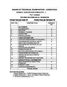
Section 2.5 Space discretization is accomplished by a boundary-fitted finite volume method. A staggered grid arrangement is used. A collocated grid arrangement is available for incompressible laminar flows. The staggered arrangement means that not all unknowns are positioned in the same points, whereas the cell-center collocated arrangement means that all the unknowns are located in the same points. Both arrangements (staggering or non-staggering) introduce extra complications, but that is of no concern to the user. The output will always contain interpolated values in the vertices of the cells. Furthermore function subroutines for boundary conditions, coefficients and initial conditions are constructed such that the user has to evaluate these quantities only in certain points, without knowing what type of points it concerns. The mathematical details with respect to the discretization can be found in the Mathematical Manual [38]. Before we discretize the equations we need a grid. In Deft we restrict ourselves to so-called structured grids. For a structured grid the region must be mapped onto a rectangle (R2 ) or a hexahedron (R3 ). As a consequence each two-dimensional region must have four ”sides” and each three-dimensional region have six ”faces”. The grid must be constructed such that it is a regular grid in the mapped region. Hence in R2 the mapped grid consists of straight cells, nx in the x-direction and ny in the y-direction. A typical example of such a mapping is shown in Figure 2.2.1. T →
Ω
G
y
↑
→ x η ξ
Figure 2.2.1: Boundary fitted co-ordinates and computational grid A region that is mapped onto one such a rectangular domain will be called a block. Of course in practical problems the regions are often too complex to map onto one single block. In that case it is necessary to subdivide the domain into sub domains each of which can be mapped on a single block. Such an ensemble of blocks will be called a multi block configuration. At this moment there is one restriction on the blocks in a multi block domain 19
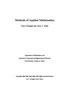
and that is that grid lines in adjacent blocks must be continuous across block boundaries. Hence a grid line at the common boundary must be present in both blocks and intersect the boundary in one point. Figure 2.2.2 shows a subdivision of a domain in six blocks, the corresponding grid is given in Figure 2.2.3.
3 5
4
2
6
1
y
Figure 2.2.2: Decomposition of region into 6 blocks
x
Figure 2.2.3: grid in multi block region
Once the grid has been defined, the finite volume method must be applied. The equations are discretized in the computational domain. Since the curved region has been mapped, the equations in the computational domain are complicated and the discretization is far from trivial. In this case there are several possibilities: 20
• The classical discretization, which is also the default discretization, is the discretization described in report 91-09 [51]. • Since the classical discretization is only applicable for fairly smooth grids an improved scheme has been developed by Wesseling and van Beek [48]. This scheme is more complicated but it is able to discretize the equations at rather non-smooth grids. • Two schemes are available with a collocated arrangement of the unknowns (See [38]).The first one (see section 5.2), corresponding to the keyword discr method=wesbeek naturally derives from the scheme developed by Wesseling and van Beek and the second one (see section 5.2) corresponding to the keyword discr method=bilinear interpolation, lays on an improvement of the previous method. It is based on bilinear interpolation. All discretization schemes may be chosen by the user.
2.2.1
Restriction for the collocated scheme based on bilinear interpolation
In case of the collocated scheme improved by bilinear interpolation, quantities at the face center of the control volumes are given by bilinear interpolation. The bilinear function is built from quantities at the cell centers. Consider the (1, 0)face in Figure 2.2.4. To keep a compact nine-point molecule, we assume that (1, 0) is surrounded by the polygons defined by (0, 0), (0, ±2), (2, ±2), (2, 0). But that is not always possible (See Figure 2.2.4). Sometimes the grid is so skewed that point (1, 0) is lying in a polygon containing other centroids. In that case, the discretization is incorrect. A solution to remedy this problem is to refine the mesh.
(4,0)
(1,0)
(2,0) (0,0)
(4,2) (2,2) (0,2)
(-2,0)
(-2,2)
Figure 2.2.4: Configuration where (1, 0) is not surrounded by (0, 0), (0, ±2), (2, ±2), (2, 0)
2.2.2
Upwind schemes
The finite volume method applied, may be considered as a type of central difference scheme. This implies that for convection-dominated flows it is possible 21
that wiggles in the solution arise. This is especially the case for the convectiondiffusion equations, where the ratio convection/diffusion may be very large. In that case upwind discretization may be necessary. In fact in case of turbulence it is hardly possible to solve the turbulence transport equations without applying upwind discretization. At this moment, four types of upwind schemes are implemented: • the standard first order upwind scheme • a hybrid central/upwind scheme • higher order upwind schemes obtained with the κ-formulation • TVD schemes with several classes of flux limiters: – Sweby Φ-limiter – R-κ limiter – MR-κ limiter – symmetric rational limiter – PL-κ limiter – MPL1-κ limiter – MPL2-κ limiter – symmetric PL-κ limiter All upwind schemes are applied in each computational direction. Hence no stream line upwinding is used. A short explanation and references of these schemes will be given below. The standard first order upwind scheme This scheme is first order accurate, but it is unconditionally monotone. Details can be found in [44]. In skewed grids, the scheme generally produces numerical cross-flow diffusion, which may result in a large error in the solution. A hybrid central/upwind scheme In an effort to combine the advantages of both central and first order upwind schemes Patankar and Spalding [33] have proposed a hybrid form of these schemes, which is based on the mesh-P´eclet number, i.e. central differencing is employed for low P´eclet and otherwise first order upwind differencing. Higher order upwind schemes Using the so-called κ-formulation of Van Leer [53], it is possible to derive a higher order upwind scheme. Assuming that the velocity ue as given in Figure 2.2.5 is positive, a general form of such a scheme may be written as 1 Te = TC + [(1 + κ)(TE − TC ) + (1 − κ)(TC − TW )] 4 22
(2.47)
W
w
C
E
e
ue Figure 2.2.5: One-dimensional finite volume used to formulate the κ-scheme where T is the unknown variable (both velocity components and scalars), the parameter −1 ≤ κ ≤ 1 indicates a specified scheme. The following often employed schemes can be obtained by setting κ as follows: κ = −1 → one-sided linear upwind difference scheme (LUDS) (2.48) κ = 0 → Fromm’s scheme 1 κ = → Cubic upwind interpolation scheme (CUI) 3 1 κ = → QUICK 2 κ = 1 → Central differencing scheme (CDS) For κ 6= 13 the local truncation error is of second order and for κ = third order.
(2.49) (2.50) (2.51) (2.52) 1 3
it is of
TVD schemes All higher order schemes mentioned above are not monotone, i.e. they can give rise to un-physical numerical oscillations. To avoid nonmonotone behaviour of the solution, a flux-limiting approach is employed [47]: 1 Te = TC + Ψ(re )(TC − TW ) 2
(2.53)
with flux limiter Ψ. The limiter argument re is the upwind ratio of consecutive solution gradients: TE − TC (2.54) re = TC − TW Note that for Ψ = 0 the first order upwind scheme is recovered. Furthermore, the κ-scheme (2.47) is implemented in the flux-limiting form, i.e., Ψκ (r) =
1 1 (1 + κ)r + (1 − κ) 2 2
(2.55)
Since no linear convection scheme of higher order accuracy can be monotone, nonlinear schemes or limiters should be employed for obtaining wiggle-free results, provided that 0 ≤ Ψ(r) ≤ min(2r, M ) (2.56) 23
where M ≥ 1 is a parameter that controls the resolution of sharp gradients, i.e. with a large value of M more accuracy near steep gradients can be obtained. The following classes of limiters are generalizations of the κ-scheme (2.55). The so-called piecewise linear κ-based (PL-κ) class of limiters, proposed in [62], has been implemented: Ψκ,M,α (r) = max[0, min(M,
1 1 (1+κ)r+ (1−κ), (2+α)r)], 2 2
M ≥ 1, −1 ≤ α ≤ 0
(2.57) The parameter α controls Ψ0 (0) and hence the amount of down-winding. This class brings together a number of flux limiters known in the literature. The Davis’ limiter used in [1] is a member of the PL-κ class with the parameters κ = −1, α = 0 and M = 1 and is identical to the BSOU scheme developed in [31]. The parameters κ = α = 0, M = 2 give a scheme which was used by Van Leer in his MUSCL approach [52]. For κ = 13 , α = 0 and M = 2 one obtains the so-called limited κ = 13 -scheme proposed by Koren [21]. The SMART scheme presented in [16] is obtained with κ = 12 , M = 4 and α = 0. By taking κ = 1, α = −1, 1 ≤ M ≤ 2 the Chakravarthy-Osher limiter is recovered, discussed, for example, in [47] and [1], which also contains the Minmod limiter (M = 1) or SOUCUP scheme proposed in [66]. Another piecewise linear class is the symmetric PL-κ limiter presented in [62], that satisfies the symmetry condition Ψ(r) = rΨ(1/r): 1 1 1 1 (1 + κ)r + (1 − κ), (1 − κ)r + (1 + κ), M r)] 2 2 2 2 (2.58) of which UMIST [25] (κ = 12 , M = 2) and MUSCL (κ = 0, M = 2) are special ones. Here 1 ≤ M ≤ 2. In [70], it has been shown that the necessary and sufficient condition for second order accuracy at smooth extrema is Ψκ,M (r) = max[0, min(M,
1 3Ψ( ) − Ψ(−1) = 2 3
(2.59)
provided that such extrema are located at cell centers. In the same paper, two modifications of (2.57) have been proposed, which satisfy (2.59) and thus enhance the accuracy of the numerical solution. The first modified class, called the MPL1-κ limiter, is given by 1 1 2 Ψκ,M,α (r) = max[0, min(2r, ), min(M, (1 + κ)r + (1 − κ), (2 + α)r)] (2.60) 3 2 2 where M ≥ 1 and −1 ≤ α ≤ 0. Observe that (2.60) and (2.57) are equivalent if −1 ≤ κ ≤ 0 and α = 0. The other modified class, to be referred to as MPL2-κ class, obeys the so-called Spekreijse’s monotonicity restriction [45]: ∃ β ∈ [−2, 0], ∃ M > 0, ∀r ∈ IR :
β ≤ Ψ(r) ≤ M
24
and
−M ≤
Ψ(r) ≤ 2+β r (2.61)
which is a less restrictive sufficient condition than (2.56) for a flux-limiting scheme (2.53) to be TVD. The modified limiter reads: 1 1 (1+κ)r+ (1−κ), (2+α)r)]+min[0, max(α, −αr)] 2 2 (2.62) where M ≥ 1 and α ∈ [−1, −κ] ∩ [−1, 0]. Clearly, the case with parameters −1 ≤ κ ≤ 0 and α = 0 is identical to (2.60). A class of piecewise linear limiters commonly used in the literature [47] is Ψκ,M,α (r) = max[0, min(M,
ΨΦ (r) = max[ 0, min(Φr, 1), min(r, Φ) ],
1≤Φ≤2
(2.63)
This so-called Sweby Φ-limiter class is not κ-dependent. Special members are Minmod (Φ = 1) and Superbee (Φ = 2) limiters. The classes of limiters presented so far are piecewise linear. The next two classes of limiters are the so-called rational κ-based (R-κ) limiters which are more smooth. The R-κ limiter is given by 2 2 (r + |r|) (−r + (3 + κ)r − κ)/(1 + r) , r ≤ 1, −1 ≤ κ < 0 ((2 + κ)r − κ)/(1 + r), r ≥ 1, −1 ≤ κ < 0 Ψκ (r) = 0≤κ≤1 (r + |r|) ((1 + κ)r + 1 − κ)/(1 + r)2 , (2.64) and has been proposed in [68, 70]. For κ = 0 in (2.64) the resulting scheme is identical to the Van Leer’s Harmonic limiter, discussed, for example, in [18], and to HLPA [65]. With κ = 12 the ISNAS limiter, as presented in [69], is obtained which is identical to NOTABLE [32]. An alternative is the MR-κ limiter that may improve the accuracy of the numerical solution, by making use of condition (2.59), and is given by r + |r|, r ≤ 13 ((8 + 9κ)r2 + (2 − 12κ)r + 2 + 3κ)/(3(1 + r)2 ), 13 ≤ r ≤ 1, −1 ≤ κ ≤ 1 Ψκ (r) = ((2 + κ)r − κ)/(1 + r), r ≥ 1, −1 ≤ κ < 0 ((8 + 9κ)r2 + (2 − 12κ)r + 2 + 3κ)/(3(1 + r)2 ), r ≥ 1, 0 ≤ κ ≤ 1 (2.65) A class of symmetric rational limiters that satisfy the monotonicity requirements (2.61) has been proposed in [62]: ΨM (r) = M
r2 + r , r2 + (M − 1)r + 1
1≤M ≤
3 2
(2.66)
M = 1 recovers the Van Albada limiter, discussed, for example, in [18], and M = 32 gives the OSPRE limiter, recently proposed in [62]. 25
In conclusion, all limiters mentioned above are nonlinear. Therefore, a limited scheme is implemented in a defect correction manner: HOS LOS o φi+1/2 = φLOS i+1/2 + (φi+1/2 − φi+1/2 )
(2.67)
where φLOS i+1/2 stands for the approximation by a lower order scheme, for example, first order upwind, and φHOS i+1/2 is the higher order approximation. The term in brackets is evaluated explicitly using the values from the previous time step, which is indicated by the superscript ‘o’.
2.3
Time integration
Since the equations to be solved are time-dependent it is necessary to use some time-integration scheme. Deft allows for three integration schemes, all of them based on the so-called θ method. Suppose one wants to solve the ordinary differential equation: dc = f (x, t), dt
(2.68)
then the θ method can be written as: cn+1 − cn = θf (x, tn+1 ) + (1 − θ)f (x, tn ) ∆t
(2.69)
where n denotes the time level and ∆t the time-step. θ must be chosen in the range 0 ≤ θ ≤ 1. For θ = 0 the method reduces to the classical explicit Euler method, for θ = 1 to the implicit Euler method. θ = 12 corresponds to the Crank Nicolson scheme. Explicit methods require a time-step restriction, since the method becomes unstable if the time-step is too large. At this moment θ = 0 has not been implemented. Fully implicit methods (θ ≥ 12 ), are unconditionally stable and hence any time-step may be used. However, an implicit scheme requires the solution of a system of linear equations at each time-step and as a consequence they are much more expensive per time-step than the explicit schemes. The Crank Nicolson scheme is second order accurate and is preferred if a timeaccurate method is required. However, a clear disadvantage of Crank Nicolson is that high frequency perturbations are not damped. For that reason a transient may be always visible if Crank Nicolson is applied. In order to damp the effect of the transient frequently values of θ greater than 0.5 are used. For example θ = 0.55 is very popular. The Euler implicit scheme may be less accurate but disturbances are damped very rapidly. Hence, if one is only interested in a stationary solution, this method is the one to use. A disadvantage of the θ-method is the fixed θ. It could be advantageous to combine a number of different θ’s per time step in such a way that second order accuracy is accomplished, and some damping is ensured as well. Two methods 26
that offer this opportunity are the fractional θ-method and the generalized θmethod. The latter is a generalization of the fractional θ-method, so we will restrict ourselves to the description of the Pkgeneralized θ-method. We rewrite equation ( 2.69) as follows, letting Σk = i=1 θi : � cn+Σ2 = cn + ∆t θ1 f (x, tn ) + θ2 f (x, tn+Σ2 ) � cn+Σ4 = cn+Σ2 + ∆t θ3 f (x, tn+Σ2 ) + θ4 f (x, tn+Σ4 ) .. .. . . � n+Σ2k = cn+Σ2k−2 + ∆t θ2k−1 f (x, tn+Σ2k−2 ) + θ2k f (x, tn+Σ2k ) c
There are two necessary conditions: 1. Σ2k = 1 for a k-stage method. This gives a first order method, and is only a scaling requirement. Pk Pk 2 2 2. i=1 θ2i−1 = i=1 θ2i to guarantee second order accuracy. A third condition is optional, but guarantees some damping: 1. θ2i−1 = 0 for at least one i ∈ 1, . . . , k. This condition includes at least one Implicit Euler step per time step. The generalized θ-method is a 3-stage method, and is therefore 3 times as expensive as the Crank-Nicolson method. However, one may choose ∆tgenθ = 3·∆tCN to accomplish similar results for both methods. A common choice for the generalized θ-method is the following ‘optimum’ for k = 3: α θ1 = θ5 = , θ3 = 0, √2 √ 3 , θ4 = α 33 θ 2 = θ6 = α 6 � �−1 2 α= 1+ √ . 3 A common choice for the fractional θ-method is the following: θ1 = θ5 = βθ,
θ3 = α(1 − 2θ),
θ2 = θ6 = αθ, 1 − 2θ , α= 1−θ 1√ 2. θ = 1− 2
θ4 = β(1 − 2θ), β=
θ 1−θ ,
With respect to the solution of the momentum equations coupled with some transport equations and or the turbulence equations, the situation is somewhat 27
more complex. In our present code we decouple the solution of momentum equations and transport equations. This means that in each time-step we start with the solution of the momentum equations coupled with the continuity equation. If coefficients depend on unknown variables at the new time level, the values at the previous time-level are used. After computing the velocity and pressure, the first transport quantity is computed, then the second and so on. Finally the turbulent quantities first k than ε or ω. A consequence of this de-coupling is that the stability of the global system may be influenced. So due to the de-coupling it is possible that a smaller time-step may be necessary than one would expect if all equations would be solved simultaneously. The turbulence equations may act on a much smaller time scale than the momentum equations. If that is the case the time step is limited due to the turbulence equations and a much smaller time step is required than one would need for the momentum equations itself. In order to avoid a large overhead it is possible to perform a sub-stepping for the turbulence equations. This means that the turbulence equations are solved with a time step that is a fraction of the global time step. This sub-stepping is only implemented in combination with the Euler implicit scheme.
2.4
Aspects with respect to the incompressibility condition
One of the main problems of the incompressibility condition is that the continuity equation does not contain the pressure, where the equation itself is strongly related to the pressure computation. As a consequence the solution of the coupled momentum equations with the continuity equation is in general everything but simple. In fact it is always necessary to take precautions in order to be able to solve the coupled equations. For time-dependent problems the pressure-correction method is one of the most popular methods to solve the problem with the continuity equation. At this moment it is the only method available in Deft. Pressure-correction may be considered as type of splitting method. In the first step the velocity is estimated using the pressure at the previous time-level. In the next step the computed velocity is projected onto the space of divergencefree vector fields. In this step a type of Poisson equation for the pressure is solved and the velocity is adapted. An important aspect of pressure correction is that during the time-stepping algorithm a term of the order of the truncation error in the time-integration scheme is neglected. Practical computations have shown that the time-step should be chosen relatively small if the solution changes rapidly, for example in case of a transient. Although, the pressure-correction method is stable if the 28
time-integration method is stable, the numerical solution may behave strangely if the gradient of the actual solution in time is large. The consequence is that the time-integration explodes (or the linear solver does not converge). The only remedy to solve this problem is to use small time-steps. However, once the solution becomes smooth in time, much larger time-steps are allowed. The pressure correction method as described above is applied such that for each time step only one prediction and one correction step is carried out. Usually this is accurate enough, and if not, the time-step should be decreased. However, in some applications, it might be wise to perform more than one iteration per time step. Such an option is available in Deft, see the keyword TIME INTEGRATION.
2.5
Aspects with respect to compressible flows
In this section certain aspects of the calculation of compressible flow, that require special attention, are explained. boundary conditions Care should be taken with the application of boundary conditions for compressible flow to have a well posed problem. We will only give an overview and refer to chapter 19 of [18] for a more elaborate discussion. We can distinguish five cases found in most common applications, where the application of the following boundary conditions leads to a well posed problem: 1. Sub-sonic inflow boundary: momentum, enthalpy prescribed 2. Supersonic inflow boundary: momentum, enthalpy and pressure prescribed 3. Sub-sonic outflow boundary: pressure, Neumann boundary condition for enthalpy prescribed 4. Supersonic outflow boundary: none prescribed 5. Solid wall boundary: freeslip or noslip for momentum, Neumann boundary condition for enthalpy prescribed Upwind discretization of convective terms In the case of compressible flow with discontinuities it is essential to use an upwind scheme for the convective terms in the momentum equation to avoid wiggles. This upwind scheme can be applied to m, as it where a convected quantity, or to the product of the quantities U and m as is commonly done in colocated schemes. It is found that the latter option gives better resolution of discontinuities. 29
Scaling of the unknowns To be able to solve the equations uniformly in Mach a scaling is applied to the pressure [2]. The pressure in the computational process is effectively the scaled perturbation of the outflow pressure: p=
p∗ − p∗out ∗2 ρ∗0 w∞
(2.70)
where p∗ and p∗out denote the dimensional pressure and outflow pressure respec∗ the stagnation density at the inflow and the velocity at tively and ρ∗0 and w∞ the inflow boundary. Furthermore all other quantities are non-dimensionalised with respect to the inflow quantities at stagnation condition [2]. These scaled quantities should be specified as boundary and initial conditions: 1
(ρu)∞ 2
(ρu)∞ h∞ pout where
1 � �− γ−1 γ−1 2 M∞ 1+ cos(α∞ ) 2 1 � �− γ−1 γ−1 2 M∞ = 1+ sin(α∞ ) 2 � �−1 γ−1 2 M∞ = 1+ 2 = 0
=
M∞
=
γ
=
α∞
=
Mach number at inflow cp cv angle of inflow with normal at inflow boundary
(2.71) (2.72) (2.73) (2.74) (2.75) (2.76) (2.77) (2.78)
Only for postprocessing purposes a reference pressure, density and velocity can be specified, which will scale the computational values back to the physical ones. If the Mach number is higher than 0.3 in the whole flow domain the scaling can be dropped and all initial and boundary conditions should be specified in a consistent dimensional form. Density Bias In the case of high Mach flow, it is essential that in the case of shocks the discretization will respect both the Rankine-Hugoniot jump relations and the entropy condition. The former is achieved by using a conservative discretization. For the latter it is necessary to introduce irreversibility in the flow. In the momentum equation this is accomplished by choosing a ( higher order) upwind scheme, in the continuity equation by choosing a form of density upwind bias. In the case of Mach-based density bias, the density is upwinded when the Mach number exceeds 0.9. If the unconditional density bias is chosen, the density 30
is always upwinded. When a higher order (limited) upwind discretization is applied to the momentum equation, the gradient based density bias should be chosen to achieve second order accuracy away from steep gradients. All types of density bias can be applied in an implicit or explicit manner. When the implicit version is applied, the pressure correction equation becomes more expensive to solve. Hence for steady state calculations the explicit version is the proper choice.
2.6
Stationary problems
At this moment Deft does not contain any special methods to compute stationary solutions. If one wants to solve a time-independent problem, the only way is to solve the instationary Navier-Stokes equations and to choose the final time so large that steady state has been reached. Whether a stationary solution has been reached can be tested in Deft with the following stopping criterion: kun+1 − un kmax ≤
� 1−λ relacckun+1 k2 + absacc , λ
with λ=
(2.79)
kun+1 − un k2 . kun − un−1 k2
The values of relacc (relative accuracy parameter) or absacc (absolute accuracy parameter) can be defined by the user, the default value is zero. It is advised to use the implicit Euler scheme in this case, since this allows for the largest time-steps. Unfortunately the combination with pressure correction may prevent the use of too large time-steps, since the solution may explode in case of a transient. The only way to solve this problem is to start with a small time-step and to enlarge the time-step after some time.
2.7
Linear solvers
After discretization of the incompressible Navier-Stokes equations various systems of linear equations have to be solved: the momentum and pressure equations and if necessary the transport and turbulence equations. In Deft these systems are always solved by iterative solution methods. The data structure used and the structured grid are very well suited for iterative solution methods of Krylov subspace-type. In order to solve the system Ax = b such a method searches for an element xk ∈ {b, Ab, ..., A(k−1) b} such that krk k = kb − Axk k is minimized in some norm. An attractive feature of these methods is that only matrix vector multiplications and basic linear algebra operations (inner products, vector updates etc. ) are used. If A is symmetric and positive definite, one of the best Krylov subspace methods 31
is the Conjugate Gradient method. However, all matrices which are used in the Deft package may be non-symmetric. For this class of matrices various Krylov subspace methods are known, where each method is optimal for a certain class of problems. For this reason several Krylov subspace methods are implemented to investigate which method should be used for a certain system. Section 2.7.1 consists of an overview of the various Krylov subspace methods and their behaviour. In general the solver, which is used as default is robust and efficient. If a better method becomes available the default is changed. It is well known that the Conjugate Gradient method only works well if a preconditioner is used. A preconditioner is a matrix P such that P ≈ A but P −1 b is much cheaper to evaluate than A−1 b. In general P should be such that the number of iterations of the original iteration method decreases considerably. The same observation holds for the other Krylov subspace methods. Therefore various preconditioners are implemented, which are discussed in Section 2.7.2. For background information we refer to [58], [55], [57].
2.7.1
Solvers
The momentum, pressure, transport, and turbulence equations are solved by iterative methods of Krylov subspace-type. Below we give references and properties of the methods implemented. LSQR [30] The easiest way to circumvent the non symmetry of the coefficient matrix is to solve the normal equations AT Ax = AT b by the Conjugate Gradient method. However this leads in general to an unstable and slow convergent method. LSQR is a stable version of the Conjugate Gradient method applied to the normal equations. For Poisson-like equations (pressure, or diffusion dominated-momentum, -transport, or -turbulence equation), LSQR is in general slow, but for convection dominated equations, which are discretized with central differences, this method can be fast. At this moment only a limited number of preconditioners are available for LSQR. BI-CGSTAB: Bi-Conjugate Gradient Stabilized [49] A generalization of the Conjugate Gradient method for non symmetric problems is the Bi-CG method. In this method two sequences of search directions are used, which are bi-orthogonal to each other. In CGS [43] one of these sequences is removed and the rate of convergence is (for many practical) examples two times as fast as Bi-CG. A more stable variant of CGS is the Bi-CGSTAB method proposed by [49]. Both methods are implemented. In general we prefer the Bi-CGSTAB method, so the CGS-method is mainly used for research reasons. An advantage of these methods is that only a limited amount of memory is required, and that no parameters have to be chosen.
32
GMRES-like methods Another generalization of the Conjugate Gradient method are GMRES-like methods. These methods have the same optimal properties with respect to the norm of the residual as the Conjugate Gradient method. However, due to the non-symmetry of the matrices all previous search directions should be stored in memory. GMRES: Generalized Minimal Residual [36] The first method in this class is the original GMRES method. Since the amount of memory increases linearly with the number of iterations it is necessary to stop the method after some iterations (in the sequel we call this number the restart value), form the approximate solution and restart the GMRES method. If the number of iterations is less than the restart value, GMRES is a very robust method. When the method is restarted, it can lose its fast convergence behaviour. A drawback is that the convergence depends critically on the restart value, so choosing the restart value too small leads to non convergence of GMRES. GCR: Generalized Conjugate Residuals [14] GCR is mathematically equivalent with GMRES. However, when unrestarted, it uses more memory than GMRES. If restarting is necessary it is possible to use other techniques (truncation) in GCR, which leads in general to a faster convergence than that of restarted GMRES. This alleviates the main drawback of GMRES. GMRESR: GMRES-Recursive [50] This method consists of an inner and an outer loop. The outer loop resembles GCR, whereas originally the inner loop consists of GMRES. Other iterative methods may be used in the inner loop. The properties of GMRESR are between that of GMRES and Bi-CGSTAB. It is a robust method and converges fast without requiring large amounts of memory. Note that GMRESR with GMRES(1) in the inner loop is equal to GCR. Finally this method is not very sensitive to variations in the restart value or the number of iterations in the inner loop. So the default values are reasonable for a wide range of problems. Directions of use For robustness the default solver is restarted GMRES for all equations. If the method is not convergent, the most robust choice is unrestarted GMRES. Another way to circumvent non convergence is to enlarge the maximal number of iterations and/or to lower the required accuracy. In many occurrences of non convergence, it appears something is wrong with the boundary conditions, coefficients or the time step used. For the pressure equation it is possible that Bi-CGSTAB is faster and/or uses less memory than the default choice. Finally the stopping criteria for the iterative methods are a compromise between efficiency and accuracy. Decreasing the required accuracy can save a considerable amount of CPU time.
33
2.7.2
The preconditioners
It appears that Krylov subspace methods are only fast converging when they are combined with a preconditioner. In this section a description is given of the preconditioners that are implemented in the Deft package. The requirements for a preconditioner P are: P ≈ A and P −1 b is cheap to evaluate. The description starts with a very simple preconditioner P , namely P is the main diagonal of A, and finishes with a complicated preconditioner P which is an incomplete LU decomposition of A. There are two different ways to use a preconditioner P . Firstly apply the method to P −1 Ax = P −1 b, which will be called preconditioning, and secondly AP −1 y = b, x = P −1 y, which will be called postconditioning. The convergence properties of the resulting preconditioned Krylov methods are approximately the same for both choices. However, when preconditioning is used the termination criterion is based on kP −1 (Axk − b)k2 , whereas if postconditioning is used the termination criterion is based on kAxk − bk2 . For this reason postconditioning is preferred, because then the termination criterion does not depend on the matrix P . We have observed examples where preconditioning needs less iterations than postconditioning, but the quality of the approximate solution was less than one may expect from the termination criterion. For background information see [58], [55], [57]. Below the implemented pre/postconditioners are specified. Diagonal If a diagonal preconditioner is used the matrix P is equal to the main diagonal of the original matrix A. ILUD The preconditioner P is an incomplete LU decomposition of the original matrix. Only the diagonal elements are adapted, the other elements of L and U are taken from the original matrix A. There are several methods to compute the diagonal elements. The original ILUD method can be modified (MILUD) in such a way that P v = Av for v = [1, 1, ..., 1]T . MILUD is fast if the solution x is slowly varying. At this moment we use RILU D = αILU D + (1 − α)M ILU D where α is a given parameter. The choice preconditioner = RILUD is implemented in the following way: suppose P is given by LLT , the iterative method is applied to L−T AL−1 y = L−T b, x = AL−1 y. 34
This enables us to use the efficient Eisenstat implementation. ILU The preconditioner is again an incomplete LU decomposition of the original matrix. Only the non-zero elements of the original matrix are adapted, so L and U have the same sparsity pattern as the original matrix. Again we use RILU = αILU + (1 − α)M ILU where α is a given parameter. This preconditioner cannot be used for the coupled momentum equations. ILU fill This preconditioner consists of an incomplete LU decomposition with fill in. The parameter fill in gives the number of diagonals allowed to become nonzero. In general the number of iterations decreases when fill in increases, however every iteration becomes more expensive. For the case that the allowed fill in is equal to the bandwidth a full LU decomposition is made and the method converges in one iteration. This preconditioning can only be used for 2 dimensional problems. It cannot be used for the coupled momentum equations. Multigrid The multigrid method is implemented as a preconditioner. This increases its robustness, whereas the extra costs for the Krylov acceleration is negligible. The method consists of a multigrid V-cycle with alternating line Jacobi as smoother. This preconditioner can be used for every number of gridpoints, so it is not necessary that these numbers are multiples of 2. Multigrid preconditioning is not available for the coupled momentum equations. Directions of use The default preconditioners are a compromise between efficiency and robustness. For the momentum equations an MILUD preconditioner is used. Although this slightly influences the termination criterion, it is more efficient since we can use the efficient Eisenstat implementation [13]. In the other equations RILU is used as postconditioner. In the pressure equation the optimal choice of α depends on the boundary conditions of the momentum equations. If Dirichlet boundary conditions are used everywhere the default choice α = 0.975 is optimal, but if on some parts of the boundary other conditions are used, then choosing α closer to one may lead to a faster convergence. For the transport and turbulence equations MILU postconditioning is the default. For a large grid-size the multigrid post conditioner can lead to a considerable decrease of CPU time for the pressure equation.
2.8
Multi-block methods
In order to solve the incompressible Navier-Stokes equations on a complicated spatial domain it is a good idea to decompose the domain into a number of 35
smaller subdomains. The solution on the subdomains depend on each other. It is the task of the multi-block (domain decomposition) method to couple the solutions of the different subdomains in such a way that the correct solution on the whole domain is obtained. This leads to an iterative algorithm that requires the repeated of problems in the subdomains. The multi-block algorithm is motivated above by geometrical reasons. Other reasons to use a multi-block approach are: parallelization or reduced memory requirements. A number of choices should be made to implement a multiblock algorithm. Below we give more details about the various choices. For background information we refer to [4].
2.8.1
Basic multi-block algorithm
In our algorithm we use non-overlapping blocks. To couple the subdomain solutions we use a Dirichlet-Dirichlet coupling. Special care is needed to handle the staggered arrangement of the unknowns. For the basic algorithm better couplings are available [4, 7]. Since we always combine the algorithm with a Krylov acceleration (where the influence of the coupling conditions is negligible) we have not implemented other coupling conditions. The multi-block algorithm can be interpreted algebraically as a Block GaussJacobi or Block Gauss-Seidel method. When the Dirichlet boundary conditions are obtained from the previous iteration we have Block Gauss-Jacobi and when the values are copied from one subdomain to another one obtains the Block Gauss-Seidel algorithm. In every multi-block iteration all subdomains are solved by an iterative method. To save CPU time it is a good idea to build the preconditioner only once and reuse it in the following multi-block iterations.
2.8.2
Subdomain solution
Two choices can be made: solve the subdomain problems accurately or inaccurately. When the subdomain problems are solved accurate enough the multiblock iteration can be applied to the interface equations. This leads to a large reduction of the vector lengths. However, this method is sensitive to the required subdomain accuracy. When the accuracy is too low the approximations do not converge to the exact solution. When the subdomain problems are solved inaccurately the iteration vectors have the same length as the solution vector on the whole domain. In general this choice is robust and more efficient than accurate solution. A special case is the so-called ILU method. Then only one iteration is done per subdomain.
2.8.3
Acceleration method
From many experiments it appears that the basic multi-block algorithm is not robust. In some applications it costs many iterations or does not converge at 36
all. To enhance this the basic multi-block method is accelerated by a Krylov subspace method: GCR [14, 50, 6]. We choose GCR because this Krylov method can be used in combination with a variable preconditioner (multi-block) [60]. Since the amount of work and memory increases with the number of GCR iterations it is necessary to restart or truncate the method. For truncation we use the Jackson-Robinson technique and by restarting we use an optimized version of GCR [56]. To speed up convergence further it is a good idea to reuse search directions of previous time-steps. For the pressure equation this leads to a large reduction of CPU time [61].
2.8.4
Parallelism
The decomposition of the global domain into subdomains leads in a natural way to a number of problems which can be solved in parallel. A parallel implementation of the accurate multi-block algorithm is presented in [5]. Also a parallel implementation of the inaccurate method is available [15]. To compare the results on one and more computers it is a good idea to use the Block Gauss-Jacobi method also on one processor, otherwise the number of iterations are different. The default (Block Gauss-Seidel) is implemented such that on each processor Block Gauss-Seidel is used, but that of course over the various processors the Block Gauss-Jacobi method is used.
2.9
Restart
In many practical applications it is necessary to write the computed solution to a file for a later restart. Reasons to do this are for example: • The necessary computation time is so long that it makes sense to save intermediate results in case of an abort. • The user wants to change the time-integration method, for example he wants to use a different value of θ. A typical example is the flow around a cylinder in which the user wants to start with one time-step Euler implicit in order to suppress the transient and after that wants to resume with a generalized θ-method or with θ = 0.5. • The user has made a computation with a set of physical constants and wishes to perform the same type of computation with a different set. In that case the solution of the preceding set might be a good initial guess. • The user has made a computation with a coarse grid and wants to do the same computation on a fine grid. The solution on the coarse grid interpolated to the fine grid may be a nice starting value, improving the convergence considerably. 37
The Deft program has its own ”data-base” to store such set of solutions. Solutions of a specific run may be identified by a so-called session identifier. At this moment this identifier is restricted to an integer number.
38
Chapter 3
The global structure of an Deft session In general the Deft session consists of four parts, which can be run separately. The four parts are • Grid generation • Pre-processing (reading and translation of the input file) • Computation (solution of the flow problem) • Post-processing (output of the results: plots and prints) The sequence of the session is always: grid generation followed by pre-processing followed by computation followed by post-processing In the Sections 3.1, 3.2, 3.3 and 3.4 the various stages are treated separately. The syntax of the input files is described in Section 3.7.
3.1
Grid generation
The first stage of an Deft job is to generate a grid. In that stage the user must decide whether he wants to use a single block approach or if multi block is necessary. Furthermore in the grid generation part it is also necessary to mark boundaries for example by a name or number in order to identify them in the pre-processing part. The reason for this is that boundary conditions must be prescribed at items that are known by some name. Grid generation may be performed with any available package. However, Deft 39
requires a special file format to be made by this grid generator and hence some ”file translator” may be necessary. The present version of the Deft incompressible pre-processor expects that the grid has been made by the SEPRAN mesh generator SEPMESH, using the special option ”isnas” or alternatively by the two-dimensional grid generator Liss. In Section 3.1.1 the usage of SEPMESH is described.
3.1.1
Usage of SEPMESH
The generation of the mesh is performed by the program SEPMESH. At this moment only a batch version is available, which requires a file with data. This file must be created by the user for example with a text editor. Program SEPMESH creates output in two ways: • SEPMESH writes to the standard output device (usually the display from which you start the program, or a standard output file). This output consists of a copy of the input file, error messages if the input is incorrect and some messages from submesh generators. • If the input is error-free and a mesh has been generated, then this mesh is written to a file named finvol.new. This file is used by the Deft preprocessor and the Deft main programs. Chapter 4 describes how a mesh is generated. SEPMESH must be used as follows: sepmesh
inputfile
sepmesh
inputfile > outputfile
or
The inputfile is the file created by the user using the text-editor. If no outputfile is specified all information (including error messages) is written directly to the screen. The output file may have any name except meshoutput, finvol.new and sepplot.∗∗ ∗, where ∗ is any digit. Example:
sepmesh pipe.msh > pipe.out.
Remark: besides the file finvol.new sepmesh also creates files sepplot.001, sepplot.002, etc. which contain plot information. So sepmesh creates output in 3 ways: • a file finvol.new containing the complete description of the mesh; 40
• files sepplot.001, sepplot.002, etc. containing information of the plots to be made; • output written to the screen or the outputfile (for example mesh.out). This output contains a hard copy of the input, error messages (if any) and some information about the mesh. How the plot information may be translated into a plot is described in Section 3.5.
3.2
Pre-processing
Once the grid has been created, the physical, mathematical and solution parameters of the problem must be specified. This means for example specification of the viscosity, the density, the boundary conditions, the type of linear solver, time integration and the turbulence model. This specification must be given with a text file. The Deft pre-processor reads this input file and interprets it. A number of possible errors in the input file is recognized by the pre-processor and in that case error messages are given. The pre-processor uses not only the input file but also the file finvol.new created by the grid generator. The Deft pre-processor has the name ISNASPRE. Program ISNASPRE creates output in two ways: • ISNASPRE writes to a file isnaspre.out. At the end of the run the tail of this file is echoed to the screen. The output file consists of a copy of the input file, and error messages or warnings if the input is incorrect. • If the input is error-free ISNASPRE creates a so-called intermediate file isnasinp.cmp. This file contains a translation from the input file to a data structure recognized by the Deft main programs. For a description of the file isnasinp.cmp consult the Deft Programmers Guide [40]. Chapter 5 describes the isnas inputfile. ISNASPRE must be used as follows: isnaspre inputfile ‘inputfile’ must have been created by the user.
3.3
Computational part of Deft
If the pre-processing phase has been completed successfully, which means that also the grid has been generated, the Deft main program can be run. Depending on the input file used in the pre-processing part, the computational part may 41
take a large amount of computing time. It is also possible to run the Deft main program parallel at several computers provided the parallel environment PVM is available. Whether or not the parallel version will be used is specified in the input file. For simple problems Deft provides a standard command: ISNASEXE. If the problem to be solved fits within the frame-work of ISNASEXE, there is no need to create or link your own main program. However, as soon as function subroutines are required to describe coefficients or boundary conditions, or if the grid is too fine to be solved by the standard program ISNASEXE it will be necessary to create and link a local program ISNASEXE. After that type: isnasexe ISNASEXE uses the files finvol.new and isnasinp.cmp created by the grid generator and the pre-processor respectively. ISNASEXE creates output in two ways: • Two files sepcomp.inf and sepcomp.out that will be used by the SEPRAN post-processor ISNASPOST. • Output is written to the file isnasexe.out containing information about the problem run as well as possible error messages and warnings. At the end of the run the tail of this file is echoed to the screen. If in some way ISNASEXE is not adequate it is necessary to create your own main program. How this must be done is described in Chapter 6. In case of a parallel environment, where the program ISNASEXE must run on several processors, the pre-processing and computational part are combined into one step. The command isnasmpi must be used to run both the preprocessor and ISNASEXE. The syntax is: isnasmpi
input_file
where input_file is the file otherwise used by ISNASPRE.
3.4
Post-processing
Once the solution has been computed, it must be post-processed in order to print or plot the results. In the present version of Deft only the SEPRAN postprocessor ISNASPOST is available. The usage of ISNASPOST is described in Section 3.4.1 42
3.4.1
Usage of ISNASPOST
In the postprocessing part of SEPRAN, the mesh created by SEPMESH is read from the file finvol.new and from the files sepcomp.inf and sepcomp.out. These files have been created in the computational part. In this section the results are produced for the user in a more suitable form: prints, plots, integrals etc. The postprocessing part is performed by the program ISNASPOST. For a description of its possibilities the reader is referred to Chapter 7. ISNASPOST is used in the same way as SEPMESH, i.e. the user creates a text input file and then runs ISNASPOST. ISNASPOST is used as follows: isnaspost inputfile >
outputfile
or isnaspost inputfile ‘inputfile is’ the file created by the user. If no outputfile is specified all information (including error messages) is written directly to the screen. ISNASPOST uses also the file created by SEPMESH (finvol.new) and those created by the Deft computational program (sepcomp.inf and sepcomp.out). ISNASPOST does not produce plots directly but produces files named sepplot.001, sepplot.002, etc. containing plot information. Since this name is the same as for the plot files produced by SEPMESH these files will be destroyed. How the plot information is translated into a plot is described in Section 3.5. Example:
3.5
isnaspost pipe.pst > pipe.out
Display of SEPRAN plots
The SEPRAN mesh generation part or the postprocessing part may generate plot files named sepplot.001, sepplot.002, sepplot.003, etc. In SEPRAN there are two ways of displaying these plots: you can make a picture at the screen, or you make a plot onto a laser printer or plotter. To display the plot on the screen use the command:
sepdisplay This interactive program tells you how many plots are available and asks you which one you want to see. sepdisplay is completely self explaining and should is by typing 43
sepdisplay
[RETURN] .
If your computer has several ways to display plot output, use the option choose plotting device to change the default plotting device into your own choice. This option gives you also the opportunity to choose the hard-copy output device. At present SEPRAN is able to produce both HPGL output (which can be used on many types of plotters and on laser printers that have an HPGL emulator build in), or Postscript output. Postscript can be used on Postscript printers only. If you use the option hard copy, in fact SEPDISPLAY does not make a hard copy but produces a file sephpgl.xxx or sepposc.xxx containing HPGL or Postscript code respectively. xxx stands for 001, 002 etc. For each new hard copy command the sequence number is increased. As soon as sepdisplay has been started it removes files with names sephpgl.xxx or sepposc.xxx. If you want to plot or print the hard copies, you have to send the files sephpgl.xxx or sepposc.xxx to the plotter or the printer. How this should be done depends on the local installation of your computer. Consult your system manager on this issue. For a UNIX environment under X-Windows there is a windows based alternative for SEPDISPLAY, the program SEPVIEW. The command SEPVIEW is activated by typing: sepview or sepview sepplot.xxx where sepplot.xxx is the file to be plotted. If sepview is used without file name, the file may be selected by the option file. Once a file is selected all files with the same basename and extension .001, .002, ... may be viewed. The first file is the file selected. SEPVIEW has the following options: Zooming in Press the left mouse button down and move the cursor upwards while pressing the button. Release the mouse button if the created rectangle is large enough. The picture within the rectangle will be drawn in the full window. Zooming out Zooming out means displaying the previous window. Zooming out is done by moving the cursor downwards while creating a rectangle. Panning Panning is done by pushing and releasing the left mouse button on the same place in the picture. The picture is panned towards the mouse position. How much the picture is panned depends on the distance between the mouse button and the middle of the picture. Hardcopy Pressing the ’Hardcopy’ button will show you a pull down menu with two possible choices. ’Postscript’ produces an encapsulated postscript 44
file .eps from the current view. An HPGL file .hpgl is generated if you press the ’HPGL’ button. is the name of the Sepran plot file and is a sequence number. It will be increased each time a new file is generated. Play / Stop / Previous / Next At the lower right corner of the plot window, there are three buttons, a left arrow, a right arrow and a push button labelled ’Play’ or ’Stop’. The name of a SEPRAN plot file is of the form nnnplot.xxx, where nnn is an arbitrary name, usually sep and xxx is a number. This number can be used to select a previous/next plot file of the same set with a higher/lower number, using the right and left arrow. If there is no plot file with a higher/lower number, the right/left arrow is disabled. To show a set of plot files as an animation, you can use the ’Play’ button. As soon as SEPVIEW has started playing, the label on the button is changed to ’Stop’ to stop the animation. As soon as the last file in the set is shown, the animation is reversed. Defaults Sepview understands all of the OSF/Motif resource names and classes as well as the ones defined below. The class name for the SEPVIEW resources is ”Sepview”. highlightThickness Specifies the thickness of the highlighting rectangle around the buttons and text areas. Default: 0 background Specifies the default background colour for drawing. Default: medium turquoise drawArea∗background Defines the drawing areas background colour. Default: turquoise An example resource for Sepview is shown below: Sepview*background: white Sepview*drawArea*background: blue
3.6
An overview of simple Deft commands
In this section we give an overview of some of the available Deft and SEPRAN commands. The following Deft/SEPRAN commands are available: • • •
sepmesh isnaspre isnasexe
(creates a grid, see Section 3.1.1) (reads and interprets the Deft input file, see Section 3.2) (performs the computational part of Deft, see Section 3.3) 45
• • •
isnaspost (performs the SEPRAN postprocessing, see Section 3.4.1) sepdisplay (displays SEPRAN plot files to the screen or produces files with hard copies, see Section 3.5) sepview (Plot SEPRAN files under X, see Section 3.5)
If you want to use the Deft/SEPRAN commands in a UNIX operating system, it is necessary to add the Deft and SEPRAN bin directory to your path. Consult your local system officer on this issue.
3.7
Syntax of input files
The ASCII input files that are used by Deft and also by SEPRAN have to satisfy syntax rules. In this section we shall explain these rules, we will use them in the following sections without explanation. The Deft and SEPRAN input files provide the following features: record A record consists of at most 80 characters. All characters behind column 80 are neglected. An input file consists of records. In Deft the division into records does not have a special meaning, hence whether items are placed in one or more records does not alter the meaning. However, to increase readability it is recommended to put each command or data item in a new record. This also simplifies maintenance. In SEPRAN it is usually necessary to start each command at a new line. separator All characters except letters, digits and the underscore sign ( ) will be regarded as separator between items. This includes also a space and end of line character. keyword A keyword is defined as a set of characters consisting of letters and the underscore sign ( ) only. The input is in case insensitive, except for strings used in output. It is not always necessary to type the complete keyword. In most cases only a limited number of characters is significant. The significant characters are written in capitals in this manual. In the input file they may be in lower case. However, it is recommended not to restrict yourself to the significant characters, since this may reduce readability. comment record Each record with a ∗ sign in the first column will be regarded as a comment record. It will be skipped when the input file is processed. comment character It is also possible to provide a comment within a record. The hash sign(#) is then used as comment character. All information behind # is treated as comment. number Numbers in records are represented in the same way as FORTRAN constants, for example: 1.0, 1.0D0, 1.0E-1, 1, .01 ; they may 46
not contain any spaces. The first character of a number must be a digit, minus sign or a point. special characters In some cases the opening and closing brackets ( and ) have a special meaning. If this is the case, this is explicitly remarked in the description of the input file. SET COMMANDS With the use of the so-called SET commands the user may give special information to the program reading the input file. These SET commands may be placed anywhere in the input file. They are active from the moment they are read. For Deft the following SET commands may be useful: SET OUTPUT OUT Once this set command is read all input read from the input file is not echoed anymore, until set output on is read. SET OUTPUT ON Reactivates the echoing of the input file. SET SKIP ON All input read after this command is skipped, which means that it is treated as comment that is not echoed. Reading is presumed in the standard way as soon as set skip off is read. This command may for example be used to prepare input files for a complete job without actually carrying out all commands. SET SKIP OFF Reactivates standard reading of the input file.
47
48
Chapter 4
Grid generation The first stage of an Deft job is to generate a grid. In that stage the user must decide whether he wants to use a single block approach or if multi block is necessary. Furthermore in the grid generation part it is also necessary to mark boundaries for example by a name or number in order to identify them in the pre-processing part. The reason is the prescription of boundary conditions at items that are known by some name. Grid generation may be performed with any available package. However, Deft requires a special file format to be made by this grid generator and hence some ”file translator” may be necessary. The present version of the Deft incompressible pre-processor expects that the grid has been made by the SEPRAN grid generator SEPMESH, using the special option ”isnas”, see Section 4.1 or alternatively by the grid generator Liss.
4.1 4.1.1
Grid generator SEPMESH General remarks
Before the grid may be created the user must keep in mind that an Deft grid consists of one or more blocks. Each block will be mapped homeomorphically onto a rectangle (2D) or a rectangular hexahedron (3D). This means that the mapping is continuous with continuous inverse. As a consequence a block in 2D has four sides and four vertices, although each side itself may contain several subsides. In R3 the grid must be restricted to a single block, since multi block has not yet been implemented for R3 . A block can not contain any holes. The sides of the 2D block or the surfaces of the 3D block may not degenerate to a quantity of lower dimension (point, side). Furthermore opposite sides in the ”rectangle” must have different points although co-ordinates may coincide. Consider for example the region in Figure 4.1.1 with four sides C1 to C4. It is 49
not allowed that curve C4 reduces to a single point. The curves C1 and C3 are identical in the sense that they have the same co-ordinates. However, with respect to the grid generation they are completely different. They will be treated as independent curves. Identification of these curves in the computational program is only possible by defining periodical boundary conditions at the curves C1 and C3. There are no limitations in the ways blocks may be coupled. Hence one side of C2
C4 C1 C3
Figure 4.1.1: C-type region with four sides C1 to C4 a block may be coupled to (parts of) sides of two other blocks. Of course in that case it is necessary to divide such a side into subsides since, if tow different blocks have a common side or subside, they should have the same name in order to be able to identify them as common. At this moment it is not allowed that the number of blocks that coincide in one point is more than four. The generation of the single block grids may be done by a standard SEPRAN sub grid generator, by a user written sub grid generator or by input from the standard input file. In this manual only the first possibility is considered. For the other cases see the SEPRAN Users Manual. The only sub grid generators allowed for Deft are RECTANGLE for two-dimensional grids and BRICK for three-dimensional grids.
4.1.2
Definition of points, curves, surfaces and volumes
For the generation of grids we define the following quantities: Points, Curves, Surfaces and Volumes Points form the basis for all other components. The user must define the main points necessary for the generation of curves. These points must be numbered sequentially from 1 onwards. After the generation of the grid they are connected to nodal point numbers. The corresponding nodal point numbers are generally not equal to the point numbers defined by the user. Curves form the one-dimensional quantities of the grids. For example lines and arcs are curves. The initial and end points of any curve must already have been defined as points. Curves have an orientation, defined by the initial and end 50
points, hence line C3 = ( P3, P4 ) is different from line C4 = ( P4, P3 ). Surfaces form the two-dimensional quantities of the grid. The boundaries of the surfaces must already have been defined as curves. The boundary of a surface must be closed in itself. Whenever in a description of a surface a curve is needed in the opposite direction of which it was defined, then its number must be preceded by a minus sign. (See Figure 4.1.4). Volumes form the three-dimensional quantities of the grid. All points, curves, surfaces and volumes must be numbered sequentially, each starting with number one. The outer and inner boundaries as defined in 2.2 must consist of points (in R1 ), points and curves (in R2 ), and points, curves and surfaces (in R3 ). The sub grids as defined in 2 must coincide with curves (in R1 ), surfaces and sometimes curves (in R2 ), or with volumes and sometimes curves and surfaces (in R3 ). Anywhere in the manuals where curves, points and surfaces are mentioned, the curves, points and surfaces generated by the grid generator are meant. Nodal points of the grid must be coupled with these points, curves and surfaces. Examples Consider the regions in Figure 4.1.2 and 4.1.3. In Figure 4.1.4 the points, curves and surfaces for these regions are defined. Points are indicated by Pk (k=1 ,2 ,,,), curves by Cl (l=1 ,2 ,,,) and surfaces by Sm (m=1 ,2 ,,,). The corresponding commands are POINTS, CURVES and SURFACES. The right upper region in FIGURE 4.1.2 is not allowed in Deft, because subblock II degenerates into a triangle.
51
I II
I III
(i)
I
(ii)
II
I
(iii)
(iv)
Figure 4.1.2: Examples of regions consisting of 1 (i),(iv) 3 (ii) and 2 (iii) subregions
I II
I III
5 outer boundaries 2 inner boundaries
6 outer boundaries
I
II
I
4 outer boundaries 1 inner boundary
8 outer boundaries 2 inner boundaries
Figure 4.1.3: Examples of inner and outer boundaries each provided with a direction
52
P6 •
P5 •
� C5
?C6 • P1
� C4
S1 C1 -
P4 • 6
C3 C2 -
• P2
• P3
C1 = (P1,P2) C2 = (P2,P3) C3 = (P3,P4) C4 = (P4,P5) C5 = (P5,P6) C6 = (P6,P1) S1:(C1,C2,C3,C4,C5,C6)
Outer boundaries: C1, C2, C3, C4, C5, C6
P6
P7
• @ @ C6 ?R S2 @ • �@ @•
C7 C9 ?S3 C1 • P1
P6
•
C6 ?
• P1
P5
•
C5 �
P5 • 6 C4
S1 P3
•
C3
P4
C2 6 • P2
C5 �
C4 �
= = = =
(P2,P3) (P4,P5) (P6,P3) (P6,P7)
Outer boundaries: C1, C2, C3, C4, C5, C8, C9 Inner boundaries: C6, C7 Attention: This region is not allowed in Deft.
C4 P5 � • C10 ? �� •P8 • C7 P9 • �� C8 • P7 P10
S1 C9 6 C1 • P2
C1 = (P1,P2) C2 C3 = (P3,P4) C4 C5 = (P5,P6) C6 C7 = (P3,P7) C8 C9 = (P7,P1) S1:(C3,C4,C5,C6) S2:(-C7,-C6,C8) S3:(C1,C2,C7,C9)
•
P4
6C3
C1 = (P1,P2) C2 = (P2,P3) C3 = (P3,P4) C4 = (P4,P5) C5 = (P5,P6) C6 = (P6,P1) C7 = (P8,P7,P10) C8 = (P10,P9,P8) C9 = (P2,P10) C10 = (P5,P8) S1:(C1,C9,C8,-C10,C5,C6) S2:(C2,C3,C4,C10,C7,-C9)
S2 C2 • Outer boundaries part 1: C1, C2, C3, C4, C5, C6 P3 Outer boundaries part 2: C7,C8 Inner boundaries: C9, C10 P4 •
C1 = (P1,P2) C2 = (P2,P3) C3 = (P3,P4) C4 = (P4,P5) C5 = (P5,P1) C6 = (P6,P9,P8) C7 = (P8,P7,P6) C8 = (P2,P8) S1:(C8,-C6,-C7,-C8,C2,C3,C4,C5,C1)
P6 S1 �� C6 • C3 • P7 ? P9 • 6 �� • C7 C8 6P8 • • • Outer boundaries part 1: C1, C2, C3, C4, C5 P1 C1 P2 C2 P3 Outer boundaries part 2: -C6, -C7 Inner boundaries: C8 53 Figure 4.1.4: Points, Curves and Surfaces
C5
4.1.3
Generation of the curves
First the user must define all points, secondly all curves and finally all surfaces. For the definition of curves, the user may specify both the number of nodal points on a curve, and the distribution of these points. For the definition of the curves the following FUNCTIONS are available: LINE< cell type >: generates a straight line from point Pi to Pj. ARC< cell type >: generates an arc from point Pi to Pj; the centroid Pc must be given. USER< cell type >: the user gives all coordinates of the nodal points on the line. CURVES: generates a curve consisting of the subsequent curves Ck, Cl, Cm. For other functions see Section 4.1.6. < cell type > is an integer which defines the type of cells along the curves to be created. In Deft only cell type = 1 is permitted. The FUNCTIONS LINE, ARC, USER and CURVES have the following shape: c1 = line c2 = arc c3=user ( c6 = curves ( ck, cl,
( p1,p2,nelm=n,ratio=r,factor=f ) ( p1,p2,pc,nelm=n,ratio=r,factor=f ) p1,p2,p3, . . . , pn ) cm, . . )
with n the number of cells in the curve. The distribution of the nodal points is given by the parameters RATIO and FACTOR: r=0: equidistant grid size (default) r=1: the last cell is f times the first cell r=2: each consecutive cell is f times the preceding cell
4.1.4
Generation of surfaces
Each surface must coincide with a subgrid (in two-dimensional problems). For the generation of nodal points and cells in the surface, a number of so-called surface generators are available. Of these surface generators only one treated in this manual. For the other ones the user is referred to the SEPRAN users manual. The surface generator described in this manual is RECTANGLE. RECTANGLE has the following characteristics: The function RECTANGLE has the following shape: S1 = RECTANGLE ( C1, C2, C3, C4) < cell type > is an integer which defines the type of cells in the surfaces to be created. In Deft only cell type = 5 is permitted, indicating that the grids consists of four-point quadrilaterals. 54
4.1.5
Input for program SEPMESH from standard input
The input for SEPMESH must be opened by the COMMAND mesh1D, mesh2D or mesh3D, depending on whether the problem is one-, two- or three-dimensional, and must be closed by the COMMAND END. COMMAND and DATA records. The records must be given in the order as specified. An option is indicated like this [ option ]. ISNAS (mandatory) COMMAND record: indicates that an Deft output file finvol.new must be created. If omitted only the SEPRAN output file meshoutput will be generated. MESHnD (mandatory) COMMAND record: opens the input for SEPMESH, and defines the dimension of the space NDIM. (NDIM = n). After the command MESHnD a number of optional commands may be given. These commands must be given between MESHnD and the mandatory command POINTS. Their mutual sequence is arbitrary. MAXPOINTS = mp (optional) mp defines the maximum number of user points that are allowed in the grid. The default value is 1000. If a smaller value is used, some arrays may be smaller, but in general this has no effect on the total space. In fact, this option is meant for those cases that 1000 user points do not suffice. MAXCURVES = mc (optional) mc defines the maximum number of curves that are allowed in the grid. The default value is 1000. Compare with MAXPOINTS. MAXSURFACES = ms (optional) ms defines the maximum number of surfaces that are allowed in the grid. The default value is 1000. Compare with MAXPOINTS. MAXVOLUMES = mv (optional) mv defines the maximum number of volumes that are allowed in the grid. The default value is 500. Compare with MAXPOINTS. POINTS (mandatory) COMMAND record: defines the points. Must be followed by data records of the type: P1 = ( x_1 , y_1 , z_1 ) P2 = ( x_2 , y_2 , z_2 ) 55
. . . Pi = ( x_i , y_i , z_i ) with i the point number and x i, y i and z i the co-ordinates of point i. For one-dimensional problems only xi is required, etc. Default values for the co-ordinates: 0. Remark: The sequence in which the points are given is arbitrary. If points are skipped, they get the co-ordinates (0,0,0) automatically. The largest number i used in Pi = . . . defines the maximal number of user points. If the user wants, he may also give the co-ordinates in polar co-ordinates instead of Cartesian co-ordinates. In that case the input is PDi = (ri , φi , zi ), with φ in degrees or PRi = (ri , φi , zi ), with φ in radians instead of Pi = (xi , yi , zi ). These co-ordinates are automatically transformed into Cartesian co-ordinates. CURVES (mandatory) COMMAND record: defines the curve. Must be followed by data records of the type: Ci Ci Ci Ci
= = = =
Ci = Ci Ci Ci Ci
= = = =
LINE ARC USER PARAM
( P1, P2, NELM=n [, RATIO=r, FACTOR=f ] ) ( P1, P2, P3, NELM=n [, RATIO=r, FACTOR=f ]) ( P1, P2, P3, . . . , Pn ) ( P1, P2, NELM=n [,INIT=t_0] [,END=t_1] [, RATIO=r, FACTOR=f ] ) SPLINE ( P1, P2, ... ,Pm, NELM=n [, RATIO=r, FACTOR=f ] [,TYPE=t [,tang=Pk, tang=Pl ] ] ) CURVES ( Ck, Cl, Cm, . . ) TRANSLATE Cj ( P1 [,P2, P3, . . . ] ) ROTATE Cj ( P1, P2, P3 [,P4, P5, . . . ] ) REFLECT Cj ( AXIS = P1, P2; P3 [,P4, P5, . . . ] )
Curves that have not been defined explicitly, will be treated as non-existing curves. These curves are not available in the SEPRAN programs. For an explanation of the various possibilities, see Section 4.1.6. SURFACES (mandatory) COMMAND record: defines the surfaces. records of the type: 56
Must be followed by data
Si = RECTANGLE (C1, C2, C3, C4 [, SMOOTH = i ] ) with Si the surface number. Surfaces that have not been defined explicitly, will be treated as nonexisting surfaces. These surfaces are not available in the SEPRAN programs. For an explanation of RECTANGLE see section 4.1.7. VOLUMES (optional) COMMAND record: defines the volumes. Must be followed by data records of the type: Vi = BRICK ( S1, S2, S3, S4, S5, S6 ) with Vi the volume number. < cell type > is an integer which defines the type of cells in the volumes to be created. In Deft only cell type = 13 is permitted, indicating that 8-point hexahedra must be created. Volumes that have not been defined explicitly, will be treated as non-existing volumes. These volumes are not available in the SEPRAN programs. For an explanation of BRICK see section 4.1.8. PLOT (optional) COMMAND record: indicates that the points, curves, the surfaces and the grid must be plotted, each on a new picture. This command record may contain data. In that case it has the following shape: PLOT ( PLOTFM = l, YFACT = y, JMARK = j, NUMSUB = n, CURVE = c, NODES = no, USERP = u, COLOUR = cl, SUPPRESS = su, ROTATE = r, EYEPOINT = (x_e,y_e,z_e) ) with PLOTFM = l the length of the plot in centimeters. Default value: depending on the computer installation, usually 15 or 20. Instead of PLOTFM = l, the user may set SCALE = s. In that case the size of the plot of the grid and sub grids is not fixed, but determined by the co-ordinates of the grid and sub grids. Hence the length in the x-direction is given by s dx and the length in the y-direction by s dy, where dx is the maximal difference of the x-coordinates in the grid or sub grid, and dy the same for the y-co-ordinates. YFACT = y: Scale factor; all y-co-ordinates are multiplied by y before plotting the grid. y 6= 1 should be used when the co-ordinates in x and y direction are of different scales, and hence the picture becomes too small. Default value: 1. JMARK = j: Indication of how the plot of the grid must be made. Possibilities: 57
0,3 Each nodal point will be marked with a star and its nodal point number. 1,4 Each nodal point will be marked with a star. Nodal point numbers will not be plotted. 2,5 Nodal points will not be marked and nodal point numbers will not be plotted. When JMARK < 3 all cell numbers will be plotted in the centroid of the cells, when JMARK ≥ 3 no cell numbers will be plotted. Default value: 5 NUMSUB = n: The sub grids with numbers ≤ NUMSUB are not plotted. Default value: 0. CURVE = c: This parameter indicates if the curves must be plotted in a separate picture. Possible values: 0 Curves are not plotted. 1 Curves are plotted without curve number. 2 Curves are plotted provided with curve number. Default value: 2. NODES = no: This parameter indicates if nodes along the curves must be plotted in the picture containing the curves. So this parameter makes only sense for c > 0. Possible values: 0 Nodes are not plotted. 1 Each node is indicated with a star-symbol (×). > 1 Each node is indicated with a symbol from the symbol table. The sequence number on the symbol table is equal to no − 1. Which symbols are stored in the symbol table depends on your plotting package. Default value: 0. SUPRESS = su: This parameter indicates if pictures must be provided with texts (su = 1) or not (su = 0). Default value: 1. ROTATE = r: This parameter indicates whether plots must be rotated over 90 degrees or not. Possibilities: 0 The plots are made such that the plotting paper used is minimal. 1 The plot is not rotated. 2 The plot is always rotated over 90 degrees. 58
Default value: 0. EYEPOINT = (xe , ye , ze ): This command makes only sense in case of a 3D region. The use of EYEPOINT indicates that a final 3D grid is plotted with hidden lines. In the case that there are many cells this plot may take much time. (xe , ye , ze ) defines the point where the observer is positioned. Remark: EYEPOINT must be written as one word. In case of a 3D grid only the sub grids are plotted, without the removal of hidden lines, except when EYEPOINT is given. For a final plot of the complete region with hidden lines removed, one may use PLOTMESH. END (mandatory) End of the input for SEPMESH.
Remark: The input must be given in the sequence: ISNAS MESH record optional commands POINTS CURVES SURFACES VOLUMES PLOT END
4.1.6
Curve generators
In this section the various curve generators will be treated. These curve generators are activated by the command CURVES in the input for the program SEPMESH. The following types of curve generators are available: LINE ARC USER PARAM SPLINE CURVES TRANSLATE ROTATE REFLECT These curve generators have the following global functions: 59
LINE generates a straight line between two end points. ARC generates an arc from begin point to end point; the centroid must be given. USERi the user gives all coordinates of the nodal points on the line. SPLINE A curve is defined by a spline through a number of points. PARAM The user defines a curve by a function subroutine FUNCCV using a parameter representation. TRANSLATE Copy a curve and translate it over a fixed distance. ROTATE Copy a curve and translate and rotate this new curve. REFLECT Make a reflection of a curve with respect to a given line. CURVES Create a new curve by combining old curves. The following options have a global meaning for each of the curves, where they may be used: NELM=n gives the number of cells that must be created along the curve (linear or quadratic depending on the value of j). RATIO=r indicates the options for distribution of the nodal points. Possibilities: r=0: equidistant grid size (default) r=1: the last cell is f times the first one. r=2: each next cell is f times the preceding one. r=3: the last cell is 1/f times the first one. r=4: each next cell is 1/f times the preceding one. FACTOR=f the factor to be used when r >1. Default: f =1. INIT=t0 gives the starting value of the parameter t along the curve. This parameter t is used in the call of subroutine FUNCCV (See the SEPRAN Users Manual 2.3.1). Default value: t0 = 0. END=t1 gives the end value of the parameter t along the curve. Default value: t1 = 1. Extended description of the various curve generators LINE The input for LINE must be given in the following way: Ci = LINE 1 ( P1, P2, NELM=n [, RATIO=r, FACTOR=f ] ) 60
This means that a straight line is generated from point P1 to point P2, with a division of cells as indicated by the options. ARC The input for ARC must be given in the following way: Ci = ARC 1 ( P1, P2, P3, NELM=n [, RATIO=r, FACTOR=f ]) When ARC is used an arc is generated from point P1 to P2 with centre P3. In R2 the sign of P3 indicates the direction of the arc. When P3 is given the arc is created counter clockwise, when -P3 is given it is created clockwise. In R3 the smallest arc from point P1 to point P2 is chosen. If the angle is exactly 180◦ , that is if the points P1, P2 and P3 are positioned on a straight line, then the direction of the arc is undefined. The arc is positioned in the plane through P1, P2 and P3. Remark: The user may give the centroid of an arc in an inaccurate way. The centroid is computed as the projection of the centroid given by the user on the line orthogonal to the line through the two end points of the arc and going through the midpoint of these two points. See Figure 4.1.5. Of course this is only possible when initial point and end point of the arc are essentially different points.
P2
P1
C
Pc
Figure 4.1.5: Computation of the centroid of an arc
USER The input for USER must be given in the following way Ci = USER 1 ( P1, P2, P3, . . . , Pn ) The curve is defined by the points P1, P2, P3, . . . , Pn in that sequence. SPLINE: The input for SPLINE must be given in the following way: 61
Ci = SPLINE 1 ( P1, P2, ... ,Pm, NELM=n [, RATIO=r, FACTOR=f ] [,TYPE=t [,tang=Pk, tang=Pl ] ] ) When SPLINE is used, the curve is defined by a cubic spline through the points P1, P2, P3, . . . , Pm. At least 3 points are required. The curve passes through all points P1, P2, .... Pm and has continuous derivative and curvature. None of the internal points P2, P3, ... Pm-1 is necessarily a nodal point. These points are not connected to nodal points either, so they can not be used in later stages of SEPRAN programs. In each sub interval [Pi, Pi + 1] the curve is a polynomial of the third degree. In SEPRAN the following SPLINE types are accessible by the option TYPE=t: t=1 The tangent of the curve is zero in the end points P1 and Pm. t=2 In [P1,P2] and [Pm − 1,Pm] the curve is a polynomial of degree 2. t=3 The spline is a closed curve, i.e. there is no begin or end point: P1 and Pm must be the same point! t=4 The spline is defined by the points P1, P2, . . . , Pn with derivatives prescribed in both begin and end point of the curve. The user must give the direction and magnitude of these derivatives by the phrase tang = Pk, tang = Pl. It is assumed that the vector Pk - P1 is the derivative in the initial point P1, and the vector Pl - Pm in the end point Pm. Hence the points Pk and Pl must have been defined already in the section points. Note that Pk is connected with the starting point and Pl with the end point. If TYPE = t is omitted, t=1 is assumed. The division of cells on the curve is defined by the parameter i, NELM=n, and (optional) RATIO=r, FACTOR=f . PARAM The input for PARAM must be given in the following way: Ci = PARAM 1 ( P1, P2, NELM=n [,INIT=t_0][,END=t_1] [, RATIO=r, FACTOR=f ] ) PARAM generates a user defined curve. The user must give the coordinates x, y and z as function of a parameter t with the aid of a user written subroutine FUNCCV. The parameter t goes from t0 to t1 . The initial point is given by P1 and the end point by P2. In this case, the length of the cells is created according to the rules defined by the parameters NELM, RATIO and FACTOR. As a consequence, the parameter t does not have to be distributed according to these same rules. Therefore, during the generation of the curves it is necessary for the program to compute the length of the curve and hence the function FUNCCV is called far more times then may be expected beforehand. 62
It is also permitted to give the distribution of the t-values over the interval. To that end 5 negative values of RATIO = r are permitted, with the following meaning: r=-1:
equidistant distribution of t, compare with r=0.
r=-2:
the last t-value is f times the first one, compare with r=1.
r=-3:
each next t-value is f times the preceding one, compare with r=2.
r=-4:
the last t-value is 1/f times the first one, compare with r=3.
r=-5:
each next t-value is 1/f times the preceding one, compare with r=4.
TRANSLATE The input for TRANSLATE must be given in the following way Ci = TRANSLATE Cj ( P1 [,P2, P3, . . . ] ) When TRANSLATE is used, the curve Ci is a copy of curve Cj translated over a distance ∆x = ((P 1i − P 1j )x , (P 1i − P 1j )y , (P 1i − P 1j )z ) with P 1i the first point on Ci and P 1j the first point on Cj. j must be smaller than i. If the points P 2, P 3, P 4, ... are given, these points correspond to the second, third etc. user points on Cj in that sequence. When these user points have co-ordinates (0,0,0), they get the new co-ordinates as computed by the translation, otherwise it is checked whether these points have the correct co-ordinates, that is if these points are indeed positioned on Ci. The point numbers i of P i may not exceed the maximal number of user points. For most applications it is necessary that both the initial and end point of a curve are identified with user points. However, if the curve to be copied consists of many user points, defining the end point of the new curve requires a large number of (possibly unnecessary) user points on this new curve. For that reason the user may identify the last user point at the new curve by preceding the point number by a minus sign. So TRANSLATE Cj ( P1, -P5 ) indicates that the begin point on curve Cj is the user point P 1 and the end point is user point P 5. If more user points are defined on the new curve, then the negative point must always be the last one in the row. ROTATE The input for ROTATE must be given in the following way: Ci = ROTATE Cj ( P1, P2, P3 [,P4, P5, . . . ] ) When ROTATE is used, the curve Ci is a copy of curve Cj translated and rotated, such that the first three user points at Ci (P1, P2 and P3) are the 63
copies of the corresponding user points at Cj. For two-dimensional grids it suffices to give two points only. If a straight line has to be translated and rotated in 3D it also suffices to give two user points on the curve Ci. These user points define the translation as well as the rotation. ROTATE may only be used for curves in a plane. j must be smaller than i. If the points P 4, P 5, P 6, ... are given, these points correspond to the fourth, fifth etc. user points on Cj in that sequence. When these user points have co-ordinates (0,0,0), they get the new co-ordinates as computed by the rotation, otherwise it will be checked whether these points have the correct co-ordinates, that is if these points are in fact positioned on Ci. The point numbers i of P i may not exceed the maximal number of user points. In the same way as for TRANSLATE the last user point in the case of ROTATE may be identified by a minus sign. REFLECT The input for REFLECT must be given in the following way: Ci = REFLECT Cj ( AXIS = P1, P2; P3, P4[, P5, . . . ] ) When REFLECT is used, curve Ci is a reflection of Cj with respect to the reflection line P 1 - P 2. At least two user points P 3 and P 4 have to be given. If the points P 5, P 6, ... are given, these points correspond to the third, fourth etcetera user points on Cj in that sequence. When these user points have co-ordinates (0,0,0), they get the new co-ordinates as computed by the reflection, otherwise it is checked whether these points have the correct co-ordinates, that is if these points are indeed positioned on Ci. The point numbers i of P i may not exceed the maximal number of user points. In the case that a curve has to be reflected in R3 instead of R2 AXIS = P 1, P 2; should be replaced by RPLANE = P 1, P 2, P 3; since in the threedimensional space a reflection plane is required. In the same way as for TRANSLATE the last user point in the case of REFLECT may be identified by a negative sign. CURVES The input for CURVES must be given in the following way: Ci = CURVES ( Ck, Cl, Cm, . . ) When CURVES is used a curve is defined by the subsequent curves Ck, Cl, Cm, ... When the sign of the curve number is positive, the positive direction will be used, otherwise (negative sign), the reversed direction of the curve will be used. The curve numbers Ci must be larger than Ck, Cl, and Cm.
4.1.7
Surface generator RECTANGLE
The surface generator RECTANGLE is called by the program SEPMESH. The user may activate RECTANGLE by data records of the type: 64
Si = RECTANGLE 5 ( C1, C2, C3, C4 [, SMOOTH = i] ) with Si the surface number, 5 the shape number of the cells created in this surface, and C1, C2, C3 and C4 the curves enclosing Si. Characteristics of RECTANGLE: Generates a subgrid that can be homeomorphically mapped onto a rectangular grid. The number of curves along the boundary must be exactly equal to four and it is assumed that N is equal to the number of cells at the first curve and M equal to the number of cells at the second one. Of course it is necessary that the number of points at the third curve is equal to the number of points at the first curve and the number of cells at the fourth curve is also equal to M. If sub curves are used, the curves along the boundary must be packed by the curve generator CURVES, which creates curves of curves. With the parameter SMOOTH it is possible to define a kind of smoothing in the grid. First the grid is generated by a algebraic method and then, if i > 0, the grid is smoothed by a so-called potential smoother. The smoothing is stopped if the relative difference between two steps in the smoothing process is less than 10−i . If SMOOTH is not given i = 0 is assumed and no smoothing takes place. Smoothing may be especially useful if the grid is used for a boundary fitted finite volume or finite difference program. Figure 4.1.6 shows the grid in an l-shaped region using the non-smooth grid generated by the following input: mesh2d isnas points p1=(0,0) p2=(1,0) p3=(1,3) p4=(4,3) p5=(4,4) p6=(0,4) curves c1 = line1(p1,p2,nelm=16) c2 = line1(p2,p3,nelm=16) c3 = line1(p3,p4,nelm=16) c4 = line1(p4,p5,nelm=16) c5 = line1(p5,p6,nelm=16) c6 = line1(p6,p1,nelm=16) c7 = curves(c2,c3) c8 = curves(c5,c6) surfaces s1 = rectangle5(c1,c7,c4,c8) plot end 65
Also in Figure 4.1.6 the result is shown once the record with RECTANGLE is replaced by: mesh2d isnas points p1=(0,0) p2=(1,0) p3=(1,3) p4=(4,3) p5=(4,4) p6=(0,4) curves c1 = line1(p1,p2,nelm=16) c2 = line1(p2,p3,nelm=16) c3 = line1(p3,p4,nelm=16) c4 = line1(p4,p5,nelm=16) c5 = line1(p5,p6,nelm=16) c6 = line1(p6,p1,nelm=16) c7 = curves(c2,c3) c8 = curves(c5,c6) surfaces s1 = rectangle5(c1,c7,c4,c8,smooth=2) plot end Remark In R3 subgrid generator RECTANGLE may only be applied in a plane.
66
Figure 4.1.6: grid in L-shaped region without and with smoothing. Examples of regions that may be subdivided by RECTANGLE Actual grids
4.1.8
Volume generator BRICK
The volume generator BRICK is called by program SEPMESH. The user may activate BRICK by data records of the type: Vi = BRICK 13 ( S1, S2, S3, S4, S5, S6 ) with Vi the volume number and S1, S2, . . . the surfaces enclosing Vi. The volume must be enclosed by exactly 6 surfaces. If sub surfaces are required the user must define surfaces of surfaces. See the SEPRAN Users Manual for a description. Characteristics of BRICK: Generates a sub mesh that can be mapped onto a rectangular (three-dimensional) grid. This rectangular region is plotted in Figure 4.1.7. The region is defined by the 6 surfaces. These surfaces must each be triangulated by the surface generator RECTANGLE. The surfaces must be given in the sequence S1, S2, . . . , S6, where S1 is defined by the face 1,2,3,4, S2 is defined by the face 1,2,6,5, 67
Computational grid N 1
N = 3,
M=5
N+! M
Number of cells along the boundary: 2 (N + M)
(M-1)N+1
NM
S3 is defined by the face 2,3,7,6, S4 is defined by the face 4,3,7,8, S5 is defined by the face 1,4,8,5, S6 is defined by the face 5,6,7,8. The numbers refer to the points in Figure 4.1.7. These surfaces must each be generated in the way as indicated above, hence S1 must start with point 1, then point 2, point 3 and point 4, etc. The parameters N, M and L correspond to the number of elements to be created along the surfaces in the following way: Curves (1,2), (5,6), (4,3), (8,7): n elements. Curves (1,4), (2,3), (5,8), (6,7): m elements. Curves (1,5), (2,6), (3,7), (4,8): l elements. The surfaces may be curved and do not have to be part of a plane. The number of elements to be created is equal to αnml where α=1 for hexahedral elements and α=6 for tetrahedral elements. Remark Instead of the surface generator RECTANGLE also the surface generators COONS and PARSURF may be used to generate the surfaces, provided the number of nodes is the same at opposite curves. In fact in these cases the underlying sub mesh generator is RECTANGLE. See the SEPRAN Users manual for details.
68
1
N M
M N
1
N 1 1
M
Coinciding first and last boundary
N M
8 7 5 4 1
6 3 2
Figure 4.1.7: Rectangular region with 6 sides
69
70
Chapter 5
Input for the computational part In this chapter we shall give a complete description of the Deft input file to be read by program ISNASPRE. This input file is a simple ASCII text file satisfying the rules described in Section 3.7. In contrast to SEPRAN files, newline characters have no special meaning except that they act as separator. Nevertheless the use of indents and newlines improves the readability and is therefore strongly recommended. Keywords in the Deft input file may be abbreviated. It is advised, however, to use full names. The significant characters are set in capitals in this manual. The input file itself is case insensitive which means that there is no difference between capitals and lower case letters. All keywords between the square brackets [ and ] may be considered as optional and hence may be neglected. In that case default values are used. In Section 5.1 the general structure of the input file is described. The description of the sub blocks is postponed to subsequent sections.
5.1
Global description of the Deft input file
The Deft input file contains a number of so-called main keywords which control the global flow of the program. Some of these main keywords define parameters, others denote the beginning of a sub block. These sub blocks define a special sort of parameters, for example all parameters associated with the linear solver or all parameters corresponding to the coefficients. Some of the main keywords are mandatory others are optional. If optional keywords are neglected, default values are used instead. The main keywords are given in the following list: 71
Keyword
Default value
NUMBER_OF_TRANsport_equations = n NUMBER_OF_COMPuters = n TIMEON / TIMEOFF OUTPut_level = n POSTTYPe = n STATionary DISCRETization TIME_integration BOUNdary_conditions COEFficients LINEar_solver INITial_conditions TURBulence MULTI_BLOCK COMPRESSIBLE FULLY_COMPRESSIBLE CAVITY COLLOcated_grid STAGGered_grid MULTI_PHase_gas_flow FREE_SURFACE_FLOW NO_TIME_LOOP MAIN_STRUCTURE PROFILE_INPUT FREQUENT_OUTPUT END_input
0 1 off 0 0 time-dependent
none
staggered_grid staggered_grid standard flow none time-dependent none none none
mandatory no no no no no no no yes yes yes no yes no no no no no no no no no no no no no no
Meaning of these keywords: NUMBER OF TRANSPORT EQUATIONS = n defines the number of transport equations that must be solved simultaneously with the momentum equations. Turbulence equations like the k and ε equations should not be included in this number since their presence is dealt with in the part treated by TURBULENCE. Transport equations are solved taking all dependent variables at the old time level. The default value for n is 0, which means that only the momentum equations, including the pressure and possibly the turbulence equations are solved. NUMBER OF COMPuters = n defines the number of processors that may be used in parallel. If this option is used, it is supposed that you have the 72
possibility to use several computers or processors in parallel and that the MPI message passing system has been installed on your computer. If n = 1, only one computer is used and the standard serial algorithm is applied. For n > 1, parallel computing is applied at the n processors available. The default value for n is 1. TIMEON / TIMEOFF These keywords indicate whether the CPU time must be printed after each main subroutine (on) or not (off). OUTPUT LEVEL = n Defines the amount of output to be produced. The following values of n may be used: n = -1: almost all output is suppressed, n = 0: standard amount of output, n > 0: extra information, depending on the value of n. At this moment n < 3 is allowed. The default value is n = 0. POSTTYPE = n Defines how the unknowns in the centroid are translated to the vertices. This parameter makes only sense for post processing purposes, since it is applied before writing the results to the output file(s). n = 0: Interpolation is performed in physical space. A Newton process is applied to detect the position of a vertex with respect to its four surrounding centroids. This approach is accurate but more expensive than the interpolation in computational space. n = 1: Interpolation is performed in computational space. In case of non-smooth grids this approach is inaccurate. The default value is n = 0. STATIONARY means that the solution to be computed is stationary. If omitted it is assumed that the solution is time-dependent. If this keyword is given it is checked if the stationary stop criterion is satisfied and if so, the computation is stopped. However, the computation performed is instationary, hence the stationary solution is reached by a time-stepping process. DISCRETIZATION This keyword indicates that the user wants to give some extra information about the space-discretization. This keyword must be followed by subkeywords containing this extra information. If omitted the standard discretization is used. See Section 5.2 TIME INTEGRATION This keyword must be followed by subkeywords containing information about the time-integration to be applied. Also 73
information as initial time, end time and time-step should be given in this part. For that reason the keyword time integration is mandatory. See Section 5.3 BOUNDARY CONDITIONS This keyword must be followed by subkeywords containing information about the boundary conditions at the external boundaries. This keyword is mandatory. See Section 5.4 COEFFICIENTS This keyword must be followed by subkeywords containing information about the coefficients of the various differential equations (momentum and transport equations) but not of the turbulence equations. This keyword is mandatory. See Section 5.5 LINEAR SOLVER This keyword must be followed by subkeywords containing information about the linear solver for the various differential equations (momentum, pressure, turbulence and transport equations). It concerns questions like which linear solver to use, which accuracy is required, what type of pre-conditioner and so-on. If omitted the default values are used. See Section 5.6 INITIAL CONDITIONS This keyword must be followed by subkeywords containing information about the initial conditions for the various equations. If omitted the default values are used, which means that all degrees of freedom are initialized to zero, except the turbulence quantities, which are set to 10−4 See Section 5.7 TURBULENCE This keyword must be followed by subkeywords containing information about the type of turbulence modeling and if necessary about the coefficients to be used. If omitted a laminar flow is assumed. See Section 5.8 MULTI BLOCK This keyword must be followed by subkeywords containing information about the multi block process for the various differential equations (momentum, pressure, turbulence and transport equations). It concerns questions like which type of algorithm to use, which accuracy is required and so-on. If omitted the default values are used. See Section 5.9 COLLOCATED GRID Indicates that the momentum equations must be solved on a collocated grid instead of a staggered grid. STAGGERED GRID Is in fact superfluous, but has been added as opposed to COLLOCATED GRID. It indicates that the momentum equations are solved on a staggered grid, which is in fact the default. COMPRESSIBLE This keyword must be followed by subkeywords containing information about the compressible flow computation. If omitted the default values are used. See Section 5.10 74
FULLY COMPRESSIBLE This keyword must be followed by subkeywords containing information about the compressible flow computation. If omitted the default values are used. See Section 5.10 The only difference with compressible is that not the pressure correction method will be used but that the continuity equation, the momentum equation and the energy equation are solved in a time-dependent semi implicit way. This option has not yet been implemented in Deft. The keywords COMPRESSIBLE and FULLY COMPRESSIBLE are mutually exclusive. CAVITY This keyword must be followed by subkeywords containing information about the cavity model. If omitted the default values are used. See Section 5.11 MULTI PHASE GAS FLOW means that the multi phase gas flow equation is solved instead of the standard equation. FREE SURFACE FLOW When this keyword is found it is assumed that at least one of the boundaries is a free-surface boundary with adapted boundary conditions. The coordinates of this boundary may change in time. The keyword may be followed by subkeywords defining information about the way the boundary must be changed in time. See Section 5.12 NO TIME LOOP If this keyword is found the solution is not only assumed to be stationary, but also a stationary solver is used. This means that no time-stepping algorithm is applied. The keywords no_time_loop and stationary are mutually exclusive. MAIN STRUCTURE This keyword is meant to have some influence on the structure of the main time-stepping subroutine. This keyword is meant for specialists only. The keyword may be followed by subkeywords defining information about the structure of the main program. See Section 5.13 PROFILE INPUT This keyword is meant to define some information with respect to a flow around a (two-dimensional) profile. At this moment it is only implemented in the unstructured finite volume program, not yet in Deft. The keyword may be followed by subkeywords defining information about the profile. See Section 5.14 FREQUENT OUTPUT This keyword is meant to define which quantities must be written in each time step to a special file. This is especially useful if some quantities must be followed in time. It concerns a limited number of quantities, complete fields are only written at the time-steps indicated by tout. At this moment it is only implemented in the unstructured finite volume 75
program, not yet in Deft. The keyword may be followed by subkeywords defining information about which quantities must be written. See Section 5.15 END INPUT defines that the end of the input has been reached. If this keyword is not available all information until the end of the file is read. Input with respect to the restart file must be given in the part INITIAL CONDITIONS (reading from the restart file) and TIME INTEGRATION (writing to the restart file).
5.2
The keyword DISCRETIZATION
The keyword DISCRETIZATION indicates that the user wants to give some extra information about the space discretization. This keyword must be followed by subkeywords containing this extra information. If omitted the standard discretization is used. The keyword may be followed by the following subkeywords: MOMentum_equations TRANSport_equation iseq TURBulence_equation iseq These subkeywords indicate to which equations the next subsubkeywords refer. In case of a transport equation or turbulence equation, the keyword must be followed by iseq. iseq denotes either a number i or the keyword ALL. If a number is given this means that the information is restricted to the corresponding equation, if ALL is given it refers to all transport or turbulence equations. These subkeywords itself may be followed by subsubkeywords that indicate whether these equations or part of it are skipped and which type of discretization is used. The following subsubkeywords are recognized: Keyword
Default value
SKIP/NOSKIP SKIP_CONTINUITY_EQUATION COUPLED/DECOUPLED CONVection/NOCONVection LIN_CONVection = type DISCR_METhod = type UPWind = type DIFFusion = type PRINT_MATrix PRINT_GMATrix PRINT_PMATrix PRINT_VECtor
noskip noskip depends on grid type convection Newton classical no standard no no no no 76
mandatory no no no no no no no no no no no no
PRINT_PVECtor PRINT_STeps = (itime1,itime2,itstep) CONSERVATIVE AXIsymmetric PRESSURE_Grad = type CONTR_VOL = type NO_TIME_DERIV NO_PRES_GRAD CONSISTMOM
no (1,1,1) no no path_six two_half_tr no no no
no no no no no no no no no
SKIP/NOSKIP If SKIP is used the complete equation is skipped. NOSKIP is the opposite of SKIP. SKIP CONTINUITY EQUATION This keyword may only be used for the momentum equations. If SKIP CONTINUITY EQUATION is used the continuity equation is skipped and the pressure and density do not change in time. This keyword is for example useful if only the momentum equations must be tested. See for an example the Burgers Equation in Section 9.10. COUPLED/DECOUPLED If COUPLED is used the momentum equations are solved as coupled system of equations. If decoupled is used the momentum equations are solved one at a time. At this moment only the combinations STAGGERED GRID and COUPLED, or COLLOCATED GRID and DECOUPLED are allowed. If a staggered grid is used the default value is COUPLED, in case of a collocated grid the default is DECOUPLED. CONVECTION/NOCONVECTION If NOCONVECTION is used, the convective terms in the momentum equations are neglected. LIN CONVECTION defines the type of linearization to be applied with respect to the convective terms. The following two values for type are available: NEWton PICard In the case of upwinding only Picard linearization is allowed except in combination with cavity. AXiSYMMETRIC defines that axi-symmetric coordinates (r,z) are used instead of Cartesian coordinates. DISCR METHOD defines the type of discretization. The following values of type are available: 77
CLAssical WESBeek REDUCed BILInear_interpolation The keyword CLASSICAL indicates that the classical Deft discretization as described in report 91-09 [51] for staggered grids is used. WESBEEK refers to the improved Wesseling and van Beek scheme either for staggered grids as explained in [48], or for collocated grids. In the latter case, a lack of accuracy may appear due to the too simple expression of the pressure gradient on non-smooth grids. The keyword REDUCED implies that the cross derivatives in the stress term are eliminated using the incompressibility condition. This is only allowed if the viscosity is constant, no turbulence model is used and the flow is incompressible. This option makes it possible to compare the results with a Cartesian code and is available for staggered grids. The keyword BILInear interpolation indicates that bilinear interpolation is used to get quantities at the cell face center of the control volumes. At this moment, it is used for collocated grids only, to evaluate accurately the gradients and the divergences, in combination with the Wesseling and VanBeek scheme which allows to calculate the stress term and the Laplacian in the pressure-correction equation. The method is explained in [27]. UPWIND defines the type of upwinding applied. The following values of type are available: NONe FIRst_order HYBrid HIGher_order, KAPpa = kappa TVD LUDs FROmm CUI QUIck MINmod SOUcup SUPerbee VAN_Leer HARmonic HLPa ISNas NOTable VAN_Albada OSPre DAVis 78
BSOu MUScl KORen SMArt UMIst NFIRst_order STREAM_FIRst, method = g OLD_NONe OLD_FIRst_o Mark that if upwind is applied only Picard linearization of the convective terms may be utilized, except in combination with cavity. The keyword NONE indicates that no upwinding is applied, hence the standard central difference scheme is used. The keyword FIRST ORDER indicates that the standard first order upwind scheme is used. The keyword HYBRID indicates that the standard hybrid central/upwind scheme is used. With the keyword HIGHER ORDER a higher order upwind scheme is activated. The keyword KAPPA defines the parameter κ which must be in the range [-1,1] and defines the type of scheme used. For example κ = 12 gives the QUICK scheme and κ = 0 the Fromm’s scheme. If omitted the default value κ = 12 is used. In order to get a higher order upwind scheme which preserves monotonicity of the solution, the keyword TVD must be chosen. This keyword must be followed by a subkeyword which specifies a flux limiter: LIMiter = limtype where limtype may take one of the following values: sweby_phi_limiter [,phi=phi] r_kappa_limiter [,kappa=k] mr_kappa_limiter [,kappa=k] symm_ratio_limiter [,mbound=m] pl_kappa_limiter [,kappa=k, mbound=m, alpha=a] mplone_kappa_limiter [,kappa=k, mbound=m, alpha=a] mpltwo_kappa_limiter [,kappa=k, mbound=m, alpha=a] symm_pl_kappa_limiter [,kappa=k, mbound=m] The keyword SWEBY PHI LIMITER indicates that one of the limiters of this type, which is specified by the parameter PHI, is used. For example Φ = 1 defines the Minmod limiter. If omitted the default value Φ = 1 is used. The keyword R KAPPA LIMITER indicates that one of the limiters of 79
this type, which is specified by the parameter KAPPA, is used. For example κ = 12 defines the ISNAS limiter. If omitted the default value κ = 12 is used. The keyword MR KAPPA LIMITER indicates that one of the limiters of this type, which is specified by the parameter KAPPA, is used. With this class a more accurate solution may be obtained. If omitted the default value κ = 12 is used. The keyword SYMM RATIO LIMITER indicates that one of the limiters of this type, which is specified by the parameter MBOUND, is used. For example M = 1 defines the Van Albada limiter. If omitted the default value M = 1 is used. The keyword PL KAPPA LIMITER indicates that one of the limiters of this type, which is specified by the parameters KAPPA, MBOUND and ALPHA, is used. For example κ = 12 , M = 4, α = 0 gives the SMART scheme. If omitted the default values κ = 12 , M = 2 and α = 0 are used. The keywords MPLONE KAPPA LIMITER and MPLTWO KAPPA LIMITER indicate that one of the limiters of these types, which is specified by the parameters KAPPA, MBOUND and ALPHA, is used. With these classes a more accurate solution may be obtained. If omitted the default values κ = 12 , M = 2 and α = 0 are used. The keyword SYMM PL KAPPA LIMITER indicates that one of the limiters of this type, which is specified by the parameters KAPPA and MBOUND, is used. For example κ = 12 , M = 2 gives the UMIST limiter. If omitted the default values κ = 12 and M = 2 are used. The keywords LUDS, FROMM, CUI, QUICK, MINMOD, SOUCUP, SUPERBEE, VAN LEER, HARMONIC, HLPA, ISNAS, NOTABLE, VAN ALBADA, OSPRE, DAVIS, BSOU, MUSCL, KOREN, SMART and UMIST are the well-known and frequently used schemes or limiters in the literature. For details and further references, see Section 2.2.2. The keyword NFIRST ORDER stands for a first order upwind approach for tudfinvol (unstructured finite volume solver). The keyword STREAM FIRST is obsolete. The keywords OLD NONE and OLD FIRST O are are only available for tudfinvol (unstructured finite volume solver). They stand for respectively central interpolation and first order upwind using an old approach to these interpolation schemes. For more information, see the manuals for tudfinvol.
DIFFUSION defines whether the diffusion terms in the transport and tur80
bulence equations are discretized in the standard way or by a special monotonous scheme. The following values of type are available: STandard HALF_Monotonous MOnotonous The keyword STANDARD indicates that the standard central difference scheme is applied, MONOTONOUS that an adapted scheme is used to get a monotonous scheme even if the cells are skewed, see [67]. However, this scheme is one-sided and thus first-order accurate. The keyword HALF Monotonous gives second-order accurate scheme which is under certain circumstances monotone, see the thesis of Demirdzic [11]. Remarks: • At this moment all the upwind schemes mentioned above, except the hybrid upwind scheme, can be used in the case of momentum equations. • In order to employ the upwind schemes for the momentum equations, Picard linearization should be used (see the keyword LIN CONVECTION). • At this moment monotonous schemes with respect to diffusion are only possible for transport and turbulence equations. • The default discretization for the convective terms in the momentum equations is the central difference scheme and in the turbulence equations is the hybrid upwind scheme. PRINT MATRIX indicates that the standard matrix must be printed. The matrix is printed for all steps indicated by PRINT STEPS. Mark that in general the matrix is large and hence printing of the matrix produces a large amount of output. This option is only meant for debug purposes. If a row of the matrix is completely zero this row will not be printed. The layout of the print may be influenced by the isnas.dbg file. PRINT GMATRIX indicates that the gradient matrix must be printed. This option makes only sense for the momentum equations. PRINT PMATRIX indicates that the pressure matrix must be printed. This option makes only sense for the momentum equations. PRINT VECTOR indicates that the standard right-hand side must be printed. The right-hand side is printed for all steps indicated by PRINT STEPS. PRINT PVECTOR indicates that the pressure right-hand side must be printed. This option makes only sense for the momentum equations. The righthand side is printed for all steps indicated by PRINT STEPS. 81
PRINT STEPS indicates that the printing defined by the options PRINT (P)VECTOR or (G/P)MATRIX must be carried for the time steps ITIME1, ITIME1+ITSTEP, ITIME1+2×ITSTEP, ... , ITIME2 CONSERVATIVE indicates that a conservative discretization of the convective terms must be used. This option is only available in 2D for the classical discretization. At this moment a conservative discretization usually does not improve the computations except in the combination of upwind and discontinuous coefficients. PRESSURE GRAD gives the user the opportunity to compute the pressure gradient using distinct methods (only for tudfinvol). The following values of type are available: PATH_Six PATH_Three AUXLine FOURPoint CONTINt Keyword PATH SIX indicates that the ordinary path-integral method using six surrounding pressure points is used. Keyword PATH Three indicates that the path-integral method using a three point stencil is used. Keyword AUXLINE indicates that auxiliary points, between the stencil points, are used. Keyword FOURPOINT indicates that the four quadrant method is used. Keyword CONTINT indicates that the pressure gradient is computed using the contour integral approach. CONTR VOL gives the user the opportunity to use different control volume for the momentum equation (only for tudfinvol). The following values are available: TWO_WHOLE_TR TWO_HALF_TR Keyword TWO WHOLE TR indicates that the control volume for a certain face consists of the two adjacent triangles. Keyword TWO HALF TR indicates that the control volume for a certain face consists of the half of the two adjacent triangles. NO TIME DERIV indicates that the time derivative is omitted. NO PRES GRAD indicates that the pressure gradient in the momentum equation is omitted. CONSISTMOM indicates that the consistency of a term in the momentum equation is investigated. 82
5.3
The keyword TIME INTEGRATION
The keyword TIME INTEGRATION indicates that the user wants to define information about the time-integration process. This keyword must be followed by subkeywords containing this information. The following subsubkeywords are recognized: Keyword
Default value
METHOD = n TINIT = t0 TEND = (t1,t2,t3,...,tl) THETA = (theta1, theta2,...) TSTEP = (dt1,dt2, ... ) TOUTInit = t TOUTEnd = t TOUTStep = DT TOUTStep = DT ABS_STATIONARY_ACCURACY = eps REL_STATIONARY_ACCURACY = eps OUTSESSION = sessionname RINIT = t0 REND = t1 RSTEP = tstep FORCE_DELETION = n RESTART = n OUTPUT = n NORM = type NSUBSTEPS_TURBULENCE = n PRESS_CORR_TIME_ITERATION ABS_PRESS_CORR_ACCURACY = eps RELAXATION_PRESS_CORR = r
THETA 0 1 1 0.1 t1 t1 dt dt 0 0 1 TOUTEND TOUTEND TOUTSTEP NO NONE DUMP LTWO 1 no 1d-4 0
mandatory no no no no no no no no no no no no no no no no no no no no no no no
METHOD = n defines the type of time-integration method to be used. The following values of n are available: THETA FRACTIONAL_STEP GENERALIZED_THETA THETA The classical θ-method with exactly one value of θ is used. For θ = 1, this is the classical Euler implicit method and for θ = 12 the Crank-Nicolson scheme. Only values of θ in the range [0.5, 1] are allowed. In this case the default value of θ is 1. FRACTIONAL STEP defines the fractional step method defined in Section 2.3. The fractional step method uses three fractional steps 83
consisting of six values of θ. The default values for θ are: θ1 = θ5 = βθ, θ3 = α(1 − 2θ), θ2 = θ6 = αθ, θ4 = β(1 − 2θ) (5.1) with
√ θ 2 1 − 2θ , β= , θ =1− α= 1−θ 1−θ 2
(5.2)
GENERALIZED THETA defines the generalized θ method defined in Section 2.3. The number of steps used in this method is implicitly defined by the input after T HET A. The number of θ-values given must be equal to two times the number of steps. If no θ-values are given the default number of three steps with the following θ-values are used. √ √ α 3 3 , θ4 = α (5.3) θ1 = θ5 = , θ3 = 0, θ2 = θ6 = α 2 6 3 with α=
�−1 � 2 . 1+ √ 3
(5.4)
TINIT = t0 defines the initial time. TEND = t1 defines the end time of the integration. If the user wants to use various time-steps ∆t, for each new time-step a separate end time must be given. The number of time-steps and the number of end times must be equal. Of course it is necessary that t1 < t2 < t3 ... TSTEP = ∆t defines the time step of the integration. If the user wants to utilize different time steps for different time intervals he may give a number of time steps and a number of end times provided these numbers are equal. For example TEND = t1 , t2 , t3 ; TSTEP = ∆t1 , ∆t2 , ∆t3 means that in the interval [t0 , t1 ] time step ∆t1 is used, in the interval [t1 , t2 ] time step ∆t2 and in the interval [t2 , t3 ] time step ∆t3 . THETA = θ defines the parameter in the θ method. In case of the fractional θ method the user must give exactly six θ-values, unless the default values are used. In case of the generalized θ-method the user must give 2 × N F RAC θvalues, where N F RAC is the number of fractional steps, unless the default values are used. TOUTINIT = t defines the first time at which output of all solutions to the output file is written. If this parameter is not defined only the last timestep is written. 84
TOUTEND = t defines the last time at which output of all solutions to the output file is written. The default value is TEND. TOUTSTEP = DT defines the frequency with which output of all solutions to the output file is written. The default value is ∆t1 , which means that all time-steps from TOUTINIT to TOUTEND are written. ABS STATIONARY ACCURACY = �1 indicates that the solution is assumed to be stationary and that the process stops as soon as steady state has been reached. This is the case when kuk+1 − uk k
or FUNC=i as described for the velocity boundary conditions and a is the sequence number of the transport equation. These boundary conditions have the following meaning: DIRICHLET The Dirichlet boundary condition prescribes the transport quantity T at the corresponding part of the boundary by T = g. NEUMANN The Neumann boundary condition prescribes the flux of the ∂T = transport quantity T at the corresponding part of the boundary by κij ni ∂x j g ROBBINS, MIXED The Robbins or mixed boundary condition prescribes a linear combination of the flux of the transport quantity T and T itself at ∂T =h the corresponding part of the boundary by αT + κij ni ∂x j WALL TEMPERATURE prescribes the Dirichlet boundary condition for the temperature T at the corresponding part of the boundary by T = g. Only meant for turbulent flows with heat transfer in which the wall temperature must be provided in order to compute the heat flux at the wall using wall functions. PERIODIC indicates that a boundary has periodical boundary conditions in exactly the same way as for the velocity. Boundary conditions for the turbulence quantities For the turbulence quantities the following types of boundary conditions may be given: K_DIrichlet = g K_NEumann = g EPS_DIrichlet = g EPS_NEumann = g EPS_ASYmptote OMEGA_DIrichlet = g OMEGA_NEumann = g OMEGA_ASYmptote K DIRICHLET prescribes a Dirichlet boundary condition for k, which means k given at the corresponding part of the boundary. 93
K NEUMANN prescribes a Neumann boundary condition for k, which means ∂k ∂n given at the corresponding part of the boundary. EPS DIRICHLET prescribes a Dirichlet boundary condition for ε, which means ε given at the corresponding part of the boundary. EPS NEUMANN prescribes a Neumann boundary condition for ε, which ∂ε given at the corresponding part of the boundary. means ∂n EPS ASYMPTOTE prescribes the asymptotic behaviour of ε near the wall. Only meant for low-Reynolds-number modeling, in which ε must asymptote to the nonzero value at the wall in order to keep the equation of turbulent energy in balance. OMEGA DIRICHLET prescribes a Dirichlet boundary condition for ω, which means ω given at the corresponding part of the boundary. OMEGA NEUMANN prescribes a Neumann boundary condition for ω, which means ∂ω ∂n given at the corresponding part of the boundary. OMEGA ASYMPTOTE prescribes the asymptotic behaviour of ω near the wall, which is given by ω= 6/β,
where Nω =
Nω ν , Y2
Y + < 5.0
(5.7)
without viscous corrections (5.8)
2/β ∗ ,
with viscous corrections
The correction can be made by the subkeyword VISCOUS CORRECTIONS as prescribed in the keyword TURBULENCE. It should be noted that grid refinement near the wall must be such that the wall-coordinate Y + , for the point nearest to the wall, must not exceed 5.0. If this ever happens, an error will occur and the run will be terminated. If for the velocity a law of the wall has been used then the boundary conditions for k and ε, are respectively ∂k =0 ∂n
(5.9)
3/4
cµ k 3/2 κY and no explicit boundary conditions should be given. ε=
(5.10)
Remark: it is necessary to give boundary conditions for the external subfaces only. Internal boundaries are treated by the multi block process. 94
5.5
The keyword COEFFICIENTS
The keyword COEFFICIENTS starts the block with information about the coefficients. This block is mandatory. The keyword may be followed by the following subkeywords: MOMentum_equations TRANSport_equation i These subkeywords indicate to which equation the next subsubkeywords refer. In case of a transport equation the keyword must be followed by a number indicating the sequence number of the transport equation. These subkeywords itself may be followed by subsubkeywords that define the coefficients. The following subsubkeywords are recognized after the keyword MOMENTUM EQUATIONS: Keyword
Default value
MU = g RHO = g FORCE1 = g FORCE2 = g FORCE3 = g MASS_FRaction = g INTERFAce_drag = g C_1 = g C_2 = g C_3 = g
1 1 0 0 0 0 0 0 0 0
mandatory no no no no no no no no no no
These coefficients have the following meaning: g may take one of the forms < number > or FUNC=i as described for the velocity boundary conditions. If FUNC = i is used a user written function subroutine is called depending on the parameter i, in the following way: 0 < i < 100 the function subroutine usfunc (6.4) is called: value = USFUNC ( i, x, y, z, t ). 100 < i < 200 the function subroutine usfunc1 (6.5) is called: value = USFUNC1 ( i-100, x, y, z, t, soluts, ndegfd ). 1000 < i < 10000 the subroutine usfilc (6.6) is called: call usfilc ( i-1000, coefs, ncoefs, icoef, ni, nj, nk, ndim, nvirtual, coor, solut, ndegfd, t ) i > 10000 corresponds to special values. 95
i = 10000 The user may fill a series of time and space dependent coefficients in one call of subroutine usfilcsp (6.7). Internally all coefficients have a sequence number. In case of the momentum equations the sequence numbers are: 1. µ 2. ρ 3. f1 4. f2 5. f3 6. � 7. β 8. C 1 9. C 2 10. C 3 The coefficients are filled according to this sequence. If the user uses for one of the coefficients the value g = 10000, he may fill a series of coefficients himself by subroutine USFILCSP. However, if for these coefficients also another input is defined (except 0), the sequence of the coefficients is important, with respect to overwriting. The best is way is to define only one coefficient with g = 10000 and to skip all coefficients that are filled by subroutine USFILCSP. The user is supposed to fill the coefficients in all cell centers in one call. The input consists of the number of cells in the various directions, the co-ordinates, the Cartesian velocity components in the vertices at the previous time level, as well as all solution vectors at the previous time level. The call is: call USFILCSP ( coefs, ncoefs, ni, nj, nk, ndim, nvirtual, coor, solut, ndegfd, t, veloc ) i = 10001 This possibility is especially meant for the construction of the righthand side of the energy equation in case of compressible flow. A user written subroutine USFILSRC is required. See (6.12) for a description. The user is supposed to fill the coefficient in all cell centers in one call. The call is:
+
call usfilsrc ( coefs, ni, nj, nk, ndim, nvirtual, coor, solut, ndegfd, time, eddy, axisym ) 96
i = 10002 This possibility is especially meant to compute the viscosity as function of other parameters. A user written subroutine USCOMPVISC is required. See (6.13) for a description. The user is supposed to fill the coefficient in all cell centers in one call. The call is: +
call uscompvisc ( coefs, eddy, ni, nj, nk, nvirtual, ndim )
MU defines the dynamical viscosity µ of the fluid. If omitted the default value 1 is used. RHO defines the density ρ of the fluid. If omitted the default value 1 is used. In case of compressible ρ is an unknown and for that reason it is necessary to give the coefficient RHO the value 1 (the default value), or no value at all. FORCE1, FORCE2, FORCE3 define the external body forces for the fluid in the Cartesian directions. For each one omitted the default values 0 is used. MASS FRAC is only used in combination with multi phase gas flow. In that case it defines the mass fraction �. INTERFACE DRAG is only used in combination with multi phase gas flow. In that case it defines the interface drag coefficient β. C 1, C 2, C 3 are at this moment only used in combination with multi phase gas flow. These coefficients define the zero-th order term in the equations, i.e. the ui equation gets the extra term +Ci ui in the equation. This option is only implemented for Cartesian grids, where the contravariant direction is identical to the Cartesian direction. The keyword TRANSPORT EQUATION a may be followed by the following subkeywords: Keyword
Default value
CAPacity = g DIFFusion = g DIFXX = g DIFXY = g DIFYY = g DIFXZ = g DIFYZ = g DIFZZ = g SOURCE = g CONStant = g
1 1 1 0 1 0 0 1 0 0 97
mandatory no no no no no no no no no no
The meaning of these coefficients is implicitly defined by the differential equation: DT + div kgrad T + CT = F, (5.11) c∗ Dt CAPACITY defines the capacity c∗ . DIFFUSION defines the diffusion k, assuming it is a scalar. DIFFXX, DIFFXY, DIFFXZ, DIFFYY, DIFFYZ, DIFFZZ define the diffusion, assuming it is a tensor quantity. SOURCE defines the source F . CONSTANT defines the constant C.
5.6
The keyword LINEAR SOLVER
The keyword LINEAR SOLVER indicates that the user wants to give some extra information about the solution of the linear systems. One may for example think about termination criteria, type of linear solver, type of preconditioner and so on. This keyword must be followed by subkeywords containing this extra information. If omitted the standard discretization is used. The keyword may be followed by the following subkeywords: MOMentum_equations TRANSport_equation iseq PRESsure_equation TURBulence_equation iseq These subkeywords indicate to which equations the next subsubkeywords refer. In case of a transport equation or turbulence equation, the keyword must be followed by either a number or the keyword ALL. If a number is given this means that the information is restricted to the corresponding equation, if ALL is given it refers to all transport or turbulence equations. These subkeywords itself may be followed by subsubkeywords that contain information about the linear solvers. The following subsubkeywords are recognized: Keyword
Default value
SOLVER = s MAXITer = n ABSAccuracy = abs RELAccuracy = rel CONDAccuracy = con DIVAccuracy = div PREConditioner = pre
GMRES 200 0 dependent 0 1e-4 dependent 98
mandatory no no no no no no no
POSTConditioner = post POLYPREConditioner = n AMOUnt_of_output = out ERRORoccurance = err GMREStart = n ORTHogonal = n MODIFY = alpha STARTVector = start RITZvalues = n PRINT_SOLution PRINT_STeps CG_RELax = omega CG_INNer = n NEUMayer NO_NEUMayer MAXLEvel = n SMOOTH_steps = n FILL_IN = n
dependent 0 0 STOP 40 dependent dependent dependent 0 no (1,1,1) 0.7 1 neumayer neumayer 0 0 8
no no no no no no no no no no no no no no no no no no
Meaning of the various subsubkeywords: SOLVER defines the type of solver. Available types for s are: CGS GMRES GCR CGSTAB MULTIgrid Explanation: CGS means standard Conjugate Gradients Squared method. GMRES means GMRES method or GMRESR(m) method. GMRESR(m) is used if Polypreconditioner is used, where m is equal to the parameter n read. GCR means the special case of GMRESR(1), which for efficiency reasons has been programmed separately. GCR may be regarded as a version of GMRES which allows for both restart and truncation. CGSTAB means the standard CGSTAB method of Sonneveld and v.d. Vorst. MULTIGRID means that the linear equations are solved by multigrid. This option has not yet been implemented. MAXITER defines the maximum number of iterations ABSACCURACY defines the absolute accuracy, if 0 (default value) a relative accuracy is used 99
RELACCURACY defines the relative accuracy, default values are: 1d-4 for the transport, turbulence and momentum equations and 1d-6 for the pressure equation. The relative accuracy is measured by measuring the decrease of the residual. This does not necessarily mean that the relative error of the solver is identical to this number. If both the absolute and relative accuracy are given, the sum of the two is used as termination criterion. CONDACCURACY makes only sense in the case of the GMRES method. It overrules the options ABSACCURACY and RELACCURACY. In this case the factor con means relative accuracy in the common sense. DIVACCURACY defines a truncation criterion for the pressure equations only. It is only used if div > 0. In that case the linear pressure solver stops if div ∗ kuk (5.12) kRi k < rel ∗ kRk + dt If rel = 0, we have:
kdivuk kuk
< div
PRECONDITIONER defines the type of preconditioner. Available values for pre are: NONE DIAGonal ILUD ILU ILU_FILL TEST Explanation: in the case of diagonal only a diagonal scaling is used ILUD uses an ILU decomposition with only the diagonal D updated. ILU uses the standard ILU(0) preconditioning, where all non-zero elements are adapted. ILU FILL uses the an ILU preconditioning, where all non-zero elements are adapted extended with a n extra diagonals. The number of extra diagonals n is given by FILL_IN = n TEST means a user written preconditioner only meant for research purposes. Default values are: In case of the momentum equation: ILUD. In case of the transport or turbulence equations: ILU. In case of the pressure equation: ILU.
100
POSTCONDITIONER defines that a postconditioner is used instead of a preconditioner. The possibilities PREConditioner and POSTConditioner exclude each other. For postconditioner the same values as for preconditioner are available. MODIFY = α is only used if an ILU or ILUD preconditioner is used. It defines whether a classical ILU(D) preconditioner is used or the modified one of Gustafsson, or some convex combination of those two. The factor α defines the weight factor in the following sense: Preconditioner = α∗ ILU + (1 − α)∗ MILU, hence α = 0 means standard method, α = 1 means Modified ILU. Default values are: In case of the momentum equation: α = 1. In case of the transport or turbulence equation: α = 1. In case of the pressure equation: α = 0.975. POLYPRECONDITIONER defines the degree of the polynomials to be taken if a polynomial preconditioner is used. 0 means no polynomial preconditioning If n > 0 an outer and an inner loop is used. The resulting method is called GMRESR. n defines the maximal number of iterations in each inner loop. The iteration method to be used in the inner loop is defined by PRECONDITIONER, MODIFY and SOLVER. At this moment only GMRES is implemented for the inner loop. Suggestion: POLYPRECONDITIONER should only be used if GMRES is used as inner iteration method. The question whether to use polypreconditioning or not is not simple to answer. A rough rule that could be used is the following: First try to run the problem without polypreconditioner. Use amount of output to get information about the number of iterations of GMRES. If more than 20 iterations are used by GMRES, it is advised to use polypreconditioning, otherwise do not use it. For more detailed information consult C. Vuik [50]. If polypreconditioning is used n=5 is a good value AMOUNT OF OUTPUT defines the amount of output (−1 ≤ n ≤ 2) ERROROCCURANCE defines how to react in case of an error. Possible values for err are: STOP RESUME STOP means stop if an error occurs. RESUME means resume the computation if possible if an error occurs . 101
GMRESTART defines after how many steps the GMRES or GCR method restarts. In the case of polypreconditioning it defines after how many steps the outer loop of GMRESR restarts. ORTHOGONAL defines after how many vectors truncation is carried out in GCR or in the case of polypreconditioning it defines after how many steps the outer loop of GMRESR truncates. Remark: if n(ortho) > n(gmrestart) no truncation is carried out. STARTVECTOR = start defines how the start vector for each iteration must be created. At this moment this possibility is meant for research possibilities only. The following values for start are available: ZERO EXPLicit PREC LINear start = ZERO means start with the null vector. start = EXPLICIT means start with an explicitly given vector. This possibility has not yet been implemented start = PREC means start with the solution at the preceding multi-block iteration (or time level in the first multi-block iteration). In the case of the pressure equation this means start with the pressure correction of the preceding time level. start = LINEAR means start with a linear extrapolation between the last two time-steps. Default values are: In case of the momentum equation: PREC. In case of the transport equation: PREC. In case of the pressure equation: PREC. Remark: in the case of a pressure equation in combination with LINEAR, the start vector is made equal to α ∗ (p(n) − p(n − 1)) where α is computed by the solver in such a way that a fast, convergence can be achieved. RITZVALUES = n, indicates that the linear solver should estimate n Ritz values after the solution has been computed. These values give insight in the solution process as well as in stability properties of the discretization. At this moment this parameter is meant for research purposes only. Suggestion: approximately 50 Ritz values give sufficient insight. PRINT SOLUTION indicates that the solution must be printed in all time steps indicated by PRINT STEPS. The solution is printed as stored in the program, that is in a staggered way and in the contravariant components that are used. 102
PRINT STEPS indicates that the printing defined by the option PRINT SOLUTION must be carried for the time steps ITIME1, ITIME1+ITSTEP, ITIME1+2×ITSTEP, ... , ITIME2 CG RELax = ω, defines the minimum value of the normed inner product between search direction and residual vector in the Bi-cgstab process. During the iteration a division by this inner product is performed. Once the value is too small the residual may grow to unacceptable values and loss of figures may be the result. This behaviour is visible in the famous peaks in many of the pictures showing the convergence behaviour of Bicgstab. Sleijpen and van der Vorst [42] propose to repair it by defining a minimum value for the inner product. This value must be between 0 and 1, and the default value is 0.7. CG INNer = n, defines the number of GMRES steps in the Bi-cgstab(l) process. The standard Bi-cgstab process consists of a Bi-CG outer loop and a GMRES(1) inner loop. According to [41] for problems with large advection Bi-cgstab(2) performs much better. l must be smaller than 16, the default value is 1. NEUMayer Neumayer [42] defined an improvement of the original CGS algorithm, which is more stable. It does not suffer so much from the erratic behaviour one often sees in the convergence pictures of CGS. The default is to use the Neumayer improvement in CGS. NO NEUMayer If No Neumayer is given as keyword, the standard CGS process is performed. FILL IN = n, defines the number of extra diagonals used to compute the ILU preconditioner in case of ILU FILL preconditioning. MAXLEVEL = n, defines the maximum number of levels in the case of multigrid preconditioning. If n=0 this number is computed in a suitable way. SMOOTH STEPS = n, defines the number of smoothing steps in the case of multigrid preconditioning. If n=0 this number is computed in a suitable way.
5.7
The keyword INITIAL CONDITIONS
The keyword INITIAL CONDITIONS indicates that the user wants to give initial conditions for some unknowns explicitly. For unknowns that have not been given any initial conditions, the initial condition 0 is assumed. In order to define the initial conditions the following subkeywords may be used: Keyword
Default value
RESTart = t
none 103
mandatory no
INSESSION = sessionname U_MOMentum = g V_MOMentum = g W_MOMentum = g TRANsport a = g PRESsure = g K_TURBulence = g EPS_TURBulence = g OMEGA_TURBulence = g REFINE = n LAMTURB = t
none 0 0 0 0 0 1e-4 1e-4 1e-4 none none
no no no no no no no no no no no
g may take one of the forms number or FUNC=i as described for the velocity boundary conditions. However, instead of a function subroutine USFUNB, the function subroutine usfuni (6.2) is used, which is called by the ISNAS program in the following way: value = USFUNI ( i, x, y, z ) INSESSION = sessionname, indicates that the computation must be resumed with the results of the session named sessionname, in order to distinguish between various sessions. At this moment sessionname is restricted to integer numbers. RESTART = t, indicates that the starting vector will be read from the restart file. The parameter t indicates the time at which the computation is resumed. U/V/W MOMENTUM = g defines the initial condition for u, v and w velocity component (in Cartesian co-ordinates) respectively. TRANSPORT a = g defines the initial condition for the ath transport quantity. PRESSURE = g defines the initial condition for the pressure. K TURBulence = g defines the initial condition for the turbulent kinetic energy k. EPS TURBulence = g defines the initial condition for the ε. OMEGA TURBulence = g defines the initial condition for the ω. REFINE = t assumes that the solution of a coarse grid has been stored in the restart file. Furthermore the mesh has been refined one times since then. The solution on the coarse grid will be interpolated to the fine grid. The parameter t has the same meaning as in RESTART = t. LAMTURB = t assumes that the solution of a laminar problem has been stored in the restart file. This laminar solution is used as starting value for the turbulent equations. The parameter t has the same meaning as in RESTART = t. 104
5.8
The keyword TURBULENCE
The keyword TURBULENCE indicates that a turbulence model will be used. If omitted the flow is assumed to be laminar. TURBULENCE may be followed by the following subkeywords: Keyword
Default value
MODEL = m LES_MODEL = l VISCOUS_CORRECTIONS = v ANISOTROPY = a KAPPA = k E = e C_MU = c SIGMA_K = s SIGMA_EPS = s CONE_EPS = c CTWO_EPS = c C_D = c SIGMA_T = s A = a E_ROUGH = e ETA_Zero = e BETARNG = b C_S = c ALPHA = a BETASTAR = b BETA = b SIGMA = s SIGMASTAR = s MOD_PRODUCTION = s CTHREE_EPS = c CTAU_ONE = c CTAU_TWO = c CTAU_THREE = c MAX_WINDOWS = m TIME_INTERVAL = t
K_EPS SMAGORINSKY NO NONE 0.41 9.0 0.09 1.0 1.3 1.44 1.92 0.08 2.0 26.6 33.0 4.38 0.012 0.1 0.556 0.09 0.075 0.5 0.5 0.0 0.05 0.0 0.0 0.0 20 1
mandatory no no no no no no no no no no no no no no no no no no no no no no no no no no no no no no
Usually the subkeyword MODEL, defining the type of turbulence model should be sufficient. The default closure constants used are those that are commonly accepted in the literature. However, the user has the option to use his own constants in the turbulence models. MODEL defines the type of turbulence model to be used. It must be followed by the type of model required. The following models are available: none 105
algebraic K_EPS RNG_K_EPS K_OMEGA LES EXT_K_EPS none no turbulence model is used, i.e. laminar flow is assumed. algebraic has not yet been implemented. K EPS defines the standard k − ε model. RNG K EPS defines the RNG k − ε model. K OMEGA defines the Wilcox k − ω model. LES means that a large eddy model is used. If the keyword LES MODEL is used this is the default value. EXT K EPS defines the extended k − ε model. LES MODEL defines the type of LES turbulence model to be used. This keyword may only be used if no turbulence model is given or if the turbulence model is set equal to LES. The following models are available: SMAGORINSKY SMAGORINSKY the SMAGORINSKY model is used. VISCOUS CORRECTIONS = v indicates whether viscous corrections must be used or not in the vicinity of a solid wall. The meaning of this subkeyword depends on the choice of the model. In the case of standard k-ε model, low-Reynolds-number effects are incorporated to reproduce the law-of-the-wall correctly. In the case of k-ω model, viscous corrections are employed for the special boundary condition for ω (see also keyword BOUNDARY CONDITIONS). The following values for v are available: YES NO YES the equations of k-ε model will be modified using the Lam-Bremhorst damping functions, or the asymptotic behaviour of ω near a wall, which is employed as a boundary condition for k-ω model, will be corrected. NO the standard k-ε model without any viscous damping functions will be employed, or the asymptotic behaviour of ω near a wall will not be corrected. ANISTROPY defines the type of anisotropic form of the eddy-viscosity concept to be used. The following models are available: 106
none SPEziale RUBinstein_barton NISizima_yoshizawa MYOng_kasagi none no anisotropic model is used, i.e. the Boussinesq hypothesis is employed. SPEZIALE defines the nonlinear model of Speziale. RUBINSTEIN BARTON gives the Rubinstein-Barton model arises from the RNG theory. NISIZIMA YOSHIZAWA means the Nisizima-Yoshizawa model based on the DIA approach. MYONG KASAGI defines the Myong-Kasagi model. C MU, SIGMA K, SIGMA EPS, CONE EPS and CTWO EPS are the empirical constants, which should be used for the standard k-ε model, RNG based k-ε model as well as the extended k-ε model. Details on the determination of these constants can be found in [24], [64] and [17], respectively. The values mentioned above are associated with the standard k-ε model. In case of the RNG model, the following values should be used: C_MU SIGMA_K SIGMA_EPS CONE_EPS CTWO_EPS
= = = = =
0.085 0.7179 0.7179 1.42 1.68
In case of the extended model, the following values should be used: C_MU SIGMA_K SIGMA_EPS CONE_EPS CTWO_EPS
= = = = =
0.09 0.75 1.15 1.35 1.9
The constants will be set according to the above mentioned values as soon as the RNG or extended model is used. ETA Zero and BETARNG are also used for the RNG model. CTHREE EPS is also used for the extended model. With respect to the Wilcox k-ω model, the following constants must be employed: ALPHA, BETASTAR, BETA, SIGMA and SIGMASTAR. For details we refer to [63].
107
KAPPA, E, A, C D and E ROUGH are the constants needed for the modeling of turbulent flow near a wall. In case of a smooth wall, the constant E will be employed, otherwise E ROUGH is used. The reason for specifying these two constants at the same time is, that different type of walls (smooth as well as rough) may be involved in one fluid problem. All of these constants, except C D and A, must be given to specify the law of the wall. The constant C D belongs to the one-equation model used in, for example, two-layer model. The constant A is needed for the specification of the so-called Van Driest mixing length. At this moment the two-layer model and Van Driest mixing length have not been implemented yet. The constant KAPPA, the so-called Von Karman constant can also be used for an algebraic model (for example the Prandtl mixing length model). C S should be used for the LES Smagorinsky model, which has not been implemented yet. SIGMA T should be used when a transport equation of temperature is involved. The constant SIGMA T is the Prandtl/Schmidt number with respect to the temperature. MOD PRODUCTION defines whether the standard expression of production term of turbulent energy is used or the Kato-Launder modification, or some convex combination of those two. The factor MOD PRODUCTION is the weight factor which lies between zero and unity. Hence, MOD PRODUCTION = 0 means standard, MOD PRODUCTION = 1 means Kato-Launder correction. If omitted the default value MOD PRODUCTION = 0 is used. CTAU ONE, CTAU TWO and CTAU THREE are the closure constants needed for the nonlinear (anisotropic) stress-strain relationship. MAX WINDOWS = m defines the maximum number of time-steps used for the time averaging procedure in the smagorinsky model. If omitted the default value 20 is used. TIME INTERVAL = t defines the time interval used for the time averaging procedure in the smagorinsky model. Mark that this value together with the present time step define the number of time steps used for the averaging. This number may not exceed the value of MAX WINDOWS. If omitted the default value 1 is used. Although it is recommended not to tune the empirical constants mentioned above, it is possible to change the values of these constants provided that the following bounds on the different constants should be employed: 0.40 ≤ κ ≤ 0.42 108
7.45 ≤ E ≤ 10.0 0.01 ≤ cµ ≤ 0.36 0.70 ≤ σk ≤ 1.40 0.70 ≤ σε ≤ 1.40 1.00 ≤ c1ε ≤ 1.55 1.50 ≤ c2ε ≤ 2.00 0.04 ≤ cd ≤ 0.15 0.50 ≤ σT ≤ 4.00 20.0 ≤ A ≤ 30.0 26.0 ≤ Erough ≤ 37.0 2.00 ≤ η0 ≤ 16.0 0.01 ≤ βRN G ≤ 0.015 0.10 ≤ Cs ≤ 0.25 0.10 ≤ α ≤ 1.0 0.04 ≤ β ∗ ≤ 0.15 0.01 ≤ β ≤ 0.1 0.50 ≤ σ ≤ 2.0 0.50 ≤ σ ∗ ≤ 2.0 0.00 ≤ modprod ≤ 1.0 0.00 ≤ c3ε ≤ 0.40
(5.13)
−5.0 ≤ cτ 1 ≤ 5.0 −5.0 ≤ cτ 2 ≤ 5.0
(5.14) (5.15)
−5.0 ≤ cτ 3 ≤ 5.0
5.9
The keyword MULTI BLOCK
The keyword MULTI BLOCK indicates that the user wants to give some extra information about the multi block process. This keyword must be followed by subkeywords containing this extra information. If omitted the standard multiblock parameters are used. The keyword may be followed by the following subkeywords: SUBDOMAIN_solution = isol SAVE_PREConditioner TYPE_OF_ALGorithm = itype MOMentum_equations TRANSport_equation i or all PRESsure_equation TURBulence_equation i or all ALL_equations 109
SUBDOMAIN SOLUTION = isol defines the way the subdomain solution is computed/approximated. The following values for isol are available: ACCurate INACCurate ILU ACCURATE means that the subdomains are assumed to be solved accurately (enough). The fact that subdomains are solved accurately means that a reduction of vector length in the acceleration is possible. INACCURATE means that the subdomains are assumed to be solved inaccurately. It is advised to lower the subdomain solution accuracy as much as possible to say 0.1. The algorithm which assumes accurate solution of subdomains is in general slower. At present, INACCURATE is the default. ILU means that the subdomain solution is approximated by applying the inverse of the subdmain ILU preconditioner to the right-hand side. This is a special case of the INACCURATE option. This method is definitely faster on a single machine than the algorithm which uses accurate solution of subdomains. SAVE PRECONDITIONER defines that the preconditioner must be built only once at in the first domain decomposition iteration. This means that the preconditioner is stored for each block and reused at every next domain decomposition iteration. The default is not to remember the preconditioner and to rebuild it each domain decomposition iteration. The default is therefore less efficient but requires less memory. TYPE OF ALGORITHM = itype defines the type of multi-block algorithm to be used. The following values for itype are available: SEQuential PARallel SEQUENTIAL means that the sequential algorithm is applied. If this algorithm is used in the case of parallel computing it means that for each processor the sequential algorithm is used but that of course over the various processors the parallel algorithm is used. PARALLEL means that the parallel algorithm is applied even if only one processor is available. This algorithm is approximately two times slower than the sequential algorithm and is in fact only available because of research purposes. The default algorithm is the sequential one. 110
...EQUATION. defines the type of equation to which the subsequent subsubkeywords should be applied. The meaning of these subkeywords is obvious. They may be followed by the subsubkeywords: Keyword METHOD = imethod AMOUnt_of_output = out MAXITer = n KRYLOV_OUter = n TRUNCATION_strategy = strategy RELAXation = r RELACcuracy = rel REUSE_SEarch = n REUSE_VAlues = yes ORTHOGONALIZATION = iortho
Default value
mandatory
accelerated 0 100 20 JACKSON_robinson 1 1e-4 0 no modified
no no no no no no no no no no
METHOD = imethod defines the type of domain decomposition algorithm to be used. The following values of imethod are available: ACCelerated STAndard STANDARD means that the standard multi-block algorithm is applied. In the case of ACCELERATED (default value) the domain decomposition process is accelerated by a GCR method. This parameter is mainly meant for research purposes. METHOD = STANDARD is only applied if the accurate subdomain solution method is chosen. AMOUNT OF OUTPUT = out, defines the amount of output. The following values for out are available: 0. ORTHOGONALIZATION = iortho indicates the type of orthogonalization scheme to be used in the multi-block process (GCR). Possible values for iortho are: modified reorthogonalized modified means the modified Gram-Schmidt process is applied. reorthogonalized the classical Gram-Schmidt process is applied with reorthogonalization. Default value: modified
5.10
The keyword COMPRESSIBLE
The keyword COMPRESSIBLE indicates that the user wants solve the compressible Navier Stokes equations. The following subkeywords may be used: Keyword GAMMA = n MACH = n VEL_Sound = n ALPha = n P_V = n P_OUT = n DENS_UPWind = method NO_DENS_UPWind NO_ENTHALPY NO_SCALING PRES_CORR_METHOD = i
Default value 1.4 0.2 330 0 0.89 0 no_dens_upwind no_dens_upwind enthalpy no_scaling 0 112
mandatory no no no no no no no no no no no
P_REF = p RHO_REF = rho VEL_REF = v ENERGY_EQUATION = e equation_of_state = e
0 1 1 enthalpy perfect_gas
no no no no no
These keywords have the following meaning: GAMMA = a gas constant equal to the specific heat at constant pressure divided by the specific heat at constant volume, in air γ = 1.4. MACH = the inlet Mach number. VEL SOUND = speed of sound, in air 330 m/s. ALPHA = inlet flow angle. P V = ratio of outlet and inlet pressure:
pout −p0 pin −p0 ,
with p0 a reference pressure.
P OUT = outlet pressure. DENS UPWIND = method = upwind-biased discretization of the density in the continuity equation, hence in the pressure correction equation, to fulfill the entropy condition. The subkeyword method is used to indicate what kind of upwinding is applied. Possible values: GRADIENT_BASED MACH_BASED UNCONDITIONAL EXPLICIT IMPLICIT EXPLICIT upwind bias is applied to the continuity equation in an explicit manner: ρn+1 − ρn + Dσ n mn+1 = 0 δt ρn σ n = upwind ρncentral
(5.16) (5.17)
IMPLICIT upwind bias is applied to the continuity equation in an implicit manner ρn+1 − ρn + Dσ n+1 mn+1 = 0 δt ρn+1 σ n+1 = upwind ρn+1 central 113
(5.18) (5.19)
GRADIENT BASED means that the density ρ is convected such that the TVD property is satisfied. The ISNAS scheme is applied. MACH BASED upwinding is applied as soon as the mach number exceeds a the value 0.9. UNCONDITIONAL A first order upwinding is applied in all cases If method is not given the default mach_based is assumed. NO DENS UPWIND = density upwinding is switched off. NO ENTHALPY means that no enthalpy equation is solved. It concerns a very special version of the compressible flow equations. NO SCALING the dimensional compressible Euler equations are solved. Nondimensionalisation is switched off. PRES CORR METHOD = i If i = 0, the compressible pressure correction method is used. If i = 1, an alternative pressure correction method is used, which better preserves contact discontinuities. P REF = p defines a reference pressure. This reference pressure is used to produce a dimensionalised pressure in the postprocessing file. RHO REF = ρ defines a reference density. This reference density is used to produce a dimensionalised density in the postprocessing file. VEL REF = u defines a reference velocity. This reference velocity is used to produce a dimensionalised velocity in the postprocessing file. ENERGY EQUATION = e defines what type of energy equation is used. This implies also what type of primary variable for the energy is utilized. Possible values for e are ENTHALPY means that the enthalpy h is used as primary energy variable. TOTAL ENTHALPY means that the total enthalpy H is used as primary energy variable. INTERNAL ENERGY means that the internal energy e is used as primary energy variable. DENS TOT ENTH means that the primary variable is the density times total enthalpy: ρH (only for tudfinvol). DENS TOT ENGY means that the primary variable is the density times total energy: ρE (only for tudfinvol). EQUATION OF STATE = e = defines what type of equation of state is used to express the relation between density, pressure and energy. Possible values for e are 114
PERFECT GAS the perfect gas law is used. USER PROVIDED a user provided equation of state is applied. The user must supply some user functions related to the equation of state. These functions are: USDRHODH (6.8), USDRHODP (6.9) and USCALCRHO (6.10). In the case that the internal energy is used as unknown, also a subroutine USCOMPINTEN must be supplied to compute the internal energy from the temperature. In this way the user may give the temperature as initial condition as well as boundary condition, and not the primary variable e. ∂ρ , which is used in the pressure correction USDRHODH computes ∂h equation. h may be either the enthalpy h, the total enthalpy H or the internal energy e, depending on the choice of energy equation. The call to this subroutine is: call usdrhodh(eddy,solut,ni,nj,nk,nvirtual,ndim,ndegfd,drhodh) USDRHODP computes ∂ρ ∂p , which is used in the pressure correction equation. The call to this subroutine is: call usdrhodp(eddy,solut,ni,nj,nk,nvirtual,ndim,ndegfd,drhodp) USCALCRHO computes ρ, as function of the previously computed solution, including the pressure The call to this subroutine is: call uscalcrho ( eddy, solut, ni, nj, nk, nvirtual, ndim, + ndegfd, ilowloop, iupploop, jlowloop, + jupploop, klowloop, kupploop ) USCOMPINTEN computes e, as function of the previously computed solution, usually the temperature The call to this subroutine is: call uscompinten ( eddy, solut, ni, nj, nk, nvirtual, ndim, ndegfd )
5.11
The keyword CAVITY
The keyword CAVITY indicates that the user wants to solve the compressible Navier Stokes equations combined with a cavity model. This keyword may only be used in combination with the keyword COMPRESSIBLE. The following subkeywords may be used: Keyword
Default value
CLIQUID CVAPOUR LOWERPRESSTRANSIT
1e-6 1e-6 1 115
mandatory no no no
UPPERPRESSTRANSIT PRESSURE_GAUSS_SEIDEL START_UP
2 none none
no no no
These keywords have the following meaning: CVAPOUR = speed of sound in the vapour phase. cliquid = speed of sound in the liquid phase lowerpresstransit = lower transit pressure of phase transition upperpresstransit = upper transit pressure of phase transition PRESSURE GAUSS SEIDEL If this keyword is found, the pressure equation is solved by a non-linear Gauss-Seidel accelerated GMRES method. START UP If this keyword is found, the cavitation calculation is started with a modified equation of state. This means that it is assumed that there is only water no cavitation. This is only necessary in a start up phase.
5.12
The keyword FREE SURFACE FLOW
The keyword FREE SURFACE FLOW indicates that the problem has at least one free surface boundary. At this moment only one algorithm to update the free boundary has been implemented. It is restricted to a stationary 2d Cartesian free boundary. The following subkeywords may be used: Keyword
Default value
METHOD = type RELAXATION = a
NONE 1
mandatory no no
These keywords have the following meaning: METHOD = type = defines the type of method that will be used to update the free boundary after each step. At this moment the following values for type are available: NONE PLAIN These subkeywords have the following meaning: NONE means that no free surface flow is computed, hence the boundary is not updated. 116
PLAIN means that the standard method is used to update the free boundary. At this moment this means that at the free boundary ∂h the boundary condition ∂h ∂t + u ∂x = v is used, with h(x) the height of the free surface, and u = (u, v) the Cartesian velocity vector. This boundary condition is discretized using a first order upwind method. Restriction: The present implementation is far from general. In fact it is assumed that we have only one block and that the region is as sketched in Figure. 5.12.1. So the top boundary is the free surface boundary free surface
y x
Figure 5.12.1: Region for free-surface flow and the grid is generated from left to right and from below to the top. This means in terms of a SEPMESH input, that C1 is the lower boundary, C2 the outflow boundary and C3 the free surface boundary. Furthermore it has been assumed that the fluid flows from left to right. RELAXATION = ω defines a relaxation factor for updating the free boundary. In order to get convergence it is necessary to define an underrelaxation parameter independent of the time step used. In our example ω = 0.1 proved to be a suitable choice.
5.13
The keyword MAIN STRUCTURE
The keyword MAIN STRUCTURE is only meant for those users that want to experiment with special algorithms. With this keyword it is possible to influence the structure of the main program. For example one can decide if an iteration over sets of equations must be carried out, or that sub-stepping for some equations must be applied. If the keyword MAIN STRUCTURE is not 117
found, the structure of the main program is completely defined by the other input parameters. However, when this keyword is used it may be necessary to define things like sub-stepping or iteration that otherwise would have been defined in other input parts. The following subkeywords may be used: GLOBAL_LOOP CLUSTER i These keywords have the following meaning: GLOBAL LOOP indicates that information about the global loop is defined. This keyword must be followed by subkeywords defining this information. CLUSTER i defines a new cluster of equations. A cluster is a conglomerate of equations (possibly consisting of one equation), which must be treated as one system with respect to loops time-stepping and so on. This keyword must be followed by subkeywords defining the cluster and containing information about the loops and so on for the cluster. Subkeywords for GLOBAL LOOP the following subkeywords are allowed Keyword SEQUENCE_OF_EQUATIONS = ( i,j,k,... ) ITERATE_INITIAL_CONDITION MIN_INITIAL_ITER = m MAX_INITIAL_ITER = m ABS_INITIAL_ACCURACY = e REL_INITIAL_ACCURACY = e MIN_STATIONARY_ITER = m MAX_STATIONARY_ITER = m
Default value
mandatory
natural sequence no 1 1 0 10e-2 0 0
no no no no no no no no
These keywords have the following meaning: SEQUENCE OF EQUATIONS = (i, j, k, ...) defines in which sequence the equations are solved per time step. ITERATE INITIAL CONDITION If this keyword is found, the program runs with the initial time step, however, without increasing the actual time, until convergence is achieved. After that the time integration actually starts. MIN INITIAL ITER = m defines the minimum number of iterations with respect to the initial condition iteration. MAX INITIAL ITER = m defines the maximum number of iterations with respect to the initial condition iteration. ABS INITIAL ACCURACY = e defines the absolute accuracy with respect to the initial condition iteration. 118
REL INITIAL ACCURACY = e defines the relative accuracy with respect to the initial condition iteration. The actual accuracy is a linear combination of both absolute and relative accuracy. MIN STATIONARY ITER = m must only be used if a stationary solution must be found. This parameter defines the minimum number of iterations. MAX STATIONARY ITER = m must only be used if a stationary solution must be found. This parameter defines the maximum number of iterations. Subkeywords for CLUSTER i the following subkeywords are allowed Keyword
Default value
EQUATIONS = ( j,k,... ) STATIONARY ABS_STATIONARY_ACCURACY = e REL_STATIONARY_ACCURACY = e MIN_STATIONARY_ITER = m MAX_STATIONARY_ITER = m nsubsteps = n
mandatory
i not 0 0 0 0 1
These keywords have the following meaning: EQUATIONS = (j, k, ...) defines which equations belong to the cluster. If omitted it is assumed that only equation i is used. STATIONARY if this keyword is found it is assumed that the present cluster must be iterated until a stationary solution is achieved for each time step. ABS STATIONARY ACCURACY = e defines the absolute accuracy with respect to the iteration for a stationary solution. REL STATIONARY ACCURACY = e defines the relative accuracy with respect to the iteration for a stationary solution. The actual accuracy is a linear combination of both absolute and relative accuracy. MIN STATIONARY ITER = m must only be used if a stationary solution must be found. This parameter defines the minimum number of iterations. MAX STATIONARY ITER = m must only be used if a stationary solution must be found. This parameter defines the maximum number of iterations. nsubsteps = n means that each time-step for the cluster is subdivided into n subtime-steps. Hence the actual time-step for the cluster is smaller than the global time step. 119
no no no no no no no
5.14
The keyword PROFILE INPUT
This keyword is meant to define some information with respect to a flow around a (two-dimensional) profile. At this moment it is only implemented in the unstructured finite volume program, not yet in Deft. The keyword may be followed by subkeywords defining information about the profile. The following subkeywords may be used: UPPER_PROFILE = Ci LOWER_PROFILE = Cj Meaning of these subkeywords: UPPER PPROFILE = Ci defines the curve number corresponding to the upper part of the profile. Mark that only one curve number may be used. This implies that if the upper part of the profile consists of several curves, these curves must be combined to a new composite curve. This option is only available if the mesh has been generated by SEPMESH. Default value: i = 1 LOWER PROFILE = Cj defines the curve number corresponding to the lower part of the profile. See also the remarks with respect to UPPER PROFILE. Default value: i = 2 With respect to profile flow, the following things must be kept in mind: • at the inflow boundary, the momentum vector must be prescribed using keywords U LEN and ANGLE. • at the outflow boundary, the boundary conditions for momentum must be SIGMANT, SIGMANN given. • the leading edge must be positioned in the origin, and the trailing edge must be positioned at the x-axis, e.g. in (1,0). • the boundary condition must be constants, i.e. not a function of time and/or position. • the upper and lower surface of the profile must each exist of one curve only.
5.15
The keyword FREQUENT OUTPUT
This is especially useful if some quantities must be followed in time. It concerns a limited number of quantities, complete fields are only written at the time-steps indicated by tout. 120
At this moment it is only implemented in the unstructured finite volume program, not yet in Deft. The keyword may be followed by subkeywords defining information about which quantities must be written. The following subkeywords may be used: FREQUENCY = f LIFT MINMAX_MACHNUMBER NUMBER_OF_SUPERSONIC_VERTICES POSITION_SONIC_POINTS DENSITY_RES_ONE DENSITY_RES_TWO DENSITY_RES_INF MOMENTUM_RES_ONE MOMENTUM_RES_TWO MOMENTUM_RES_INF ENTHALPY_RES_ONE ENTHALPY_RES_TWO ENTHALPY_RES_INF Meaning of these subkeywords: FREQUENCY = f defines the frequency with which this output is written to file sepcomp.freq. f ≥ 1 defines the time steps at which the frequent output is written. If f = 1 each time step information is written, if f = 2 only the odd time steps and so on. Default value: f = 1 LIFT If this subkeyword is found both the lift and the drag of a profile will be written to the output file. This keyword makes only sense in combination with the keyword PROFILE. If omitted the lift and drag are not written. MINMAX MACHNUMBER The minimum and maximum Mach numbers in the region will be written. This keyword makes only sense in combination with the keyword COMPRESSIBLE. If omitted the minimum and maximum Mach numbers are not written. NUMBER OF SUPERSONIC VERTICES The number of supersonic vertices in the region will be written. This keyword makes only sense in combination with the keyword COMPRESSIBLE. If omitted the number will not be written. POSITION SONIC POINTS The position of the sonic points along the profile will be written. Theoretically there are at most 2 sonic points at each side of the profile, hence 4 positions are written. In each step 4 coordinates are written defining the relative x-position along 121
the profile, where the profile is scaled from x = 0 to x = 1. If during a step more than 2 sonic points along a side are found, only the first two found are written. This keyword makes only sense in combination with the keywords COMPRESSIBLE and PROFILE. If omitted the positions are not written. DENSITY RES ONE The quantity ||ρn+1 − ρn ||1 , with n indicating the time-level, is written to file. For definitions of the norm, see below. If omitted this quantity is not written. DENSITY RES TWO The quantity ||ρn+1 − ρn ||2 , with n indicating the time-level, is written to file. For definitions of the norm, see below. If omitted this quantity is not written. DENSITY RES INF The quantity ||ρn+1 − ρn ||∞ , with n indicating the time-level, is written to file. For definitions of the norm, see below. If omitted this quantity is not written. MOMENTUM RES ONE The quantity ||mn+1 − mn ||1 , with n indicating the time-level, is written to file. For definitions of the norm, see below. If omitted this quantity is not written. MOMENTUM RES TWO The quantity ||mn+1 − mn ||2 , with n indicating the time-level, is written to file. For definitions of the norm, see below. If omitted this quantity is not written. MOMENTUM RES INF The quantity ||mn+1 − mn ||∞ , with n indicating the time-level, is written to file. For definitions of the norm, see below. If omitted this quantity is not written. ENTHALPY RES ONE The quantity ||hn+1 − hn ||1 , with n indicating the time-level, is written to file. For definitions of the norm, see below. If omitted this quantity is not written. ENTHALPY RES TWO The quantity ||hn+1 − hn ||2 , with n indicating the time-level, is written to file. For definitions of the norm, see below. If omitted this quantity is not written. ENTHALPY RES INF The quantity ||hn+1 − hn ||∞ , with n indicating the time-level, is written to file. For definitions of the norm, see below. If omitted this quantity is not written. The following definitions of norms, with u = (u1 , u2 , . . . , un ), are used: • 1 norm:
Pn ||u||1 =
• 2 norm:
i=1
|ui |
n
r Pn ||u||2 =
122
i=1
n
u2i
(5.20)
(5.21)
• ∞ norm:
||u||∞ = max(|ui |)
123
(5.22)
124
Chapter 6
Creating your own main program In many applications it is sufficient to use the command ISNASEXE and there is no need to create a main program. However, sometimes ISNASEXE does not supply enough flexibility for your purposes. Reasons for creating your own main program are for example: • It is necessary to add a function subroutine because one of the boundary conditions, one of the coefficients or perhaps the initial conditions depend on space or time. • The buffer space used by program ISNASEXE is insufficient for your application. If this is the case isnasexe returns with a message. • You are extending, changing or debugging isnasexe. This is only meant for developers and is described in the Programmers Guide [40]. In Section 6.1 it is described how you make your local main program ISNASEXE. The function subroutines that must be provided by the user in case of variable coefficients, boundary conditions or initial conditions are described in the Sections 6.2, 6.3, 6.4, 6.5 and 6.6.
6.1
How to create and run a local program ISNASEXE in a serial environment
The creation of a main program in Deft is relatively simple. The name of the main program may be chosen freely. However, there is one exception. In the case of a parallel environment, only the name isnasexe may be used, due to some scripts necessary to use mpi. This restriction is only temporarily. In general the main program has the following shape: 125
program example implicit none integer nbuffr parameter( nbuffr = 5000000 ) integer ibuffr common ibuffr(nbuffr) call is_main ( nbuffr ) end
function usfunx ( .... ) end subroutine usfilx ( .... ) end
The program name ”example” may be replaced by any other suitable name. The declarations concerning IBUFFR and NBUFFR define the length of the buffer array to be used by Deft. In this example the default length 5000000 has been used. However, if the buffer length is insufficient, this number must be enlarged. Subroutine IS MAIN is the actual main Deft subroutine. It requires the declared length of array IBUFFR as only parameter. If function subroutines must be provided, the simplest way is to put them in the same file as the main program, just behind this main program. Only the subroutines actually written by the user should be supplied. The function usf unx and the subroutine usf ilx used in the example above represent these user subroutines. The actual program isnasexe can be put into your directory by the command: isget isnasexe This command copies the standard isnasexe program into your directory with the name isnasexe.f. The next step is to adapt this program for your own purposes, and add those user subroutines that are required for the application. It is a good practice to rename the file isnasexe.f to a new name that has something to do with the application, for example channel.f. It is advised to use the same name in the program statement. Once the program has been created it must be compiled and linked. This must 126
be performed by the command islink in the following way: islink isnasexe where isnasexe stands for the name of the fortran file containing the main program, without the extension .f. The islink commands compiles the program isnasexe including all user subroutines provided in this file. After successful compilation the program isnasexe is linked with the subroutines provided, all files with the extension .o in the subdirectory, and of course the Deft libraries. The files with extension .o are supposed to be compiled before by a FORTRAN or possibly C-compiler. The file isnasexe.o itself is removed. The result of the islink command is an executable with the name isnasexe, provided compilation and linking have been carried out successfully. To run this executable, simply type its name, for example: isnasexe This program will run provided the grid has been generated before and the Deft pre-processor has been applied and no errors are generated. If Deft is run in a parallel environment on several computers, then it is necessary to link isnasexe first and after that run isnasmpi with an input file as described in Section 3.3. In that case the name of the main program is restricted to isnasexe.
6.2
Function subroutine usfuni
Description Only if the initial conditions are not constant throughout the domain it is necessary to provide the user written subroutine USFUNI. Heading function usfuni ( ichoice, x, y, z ) Parameters integer ichoice double precision usfuni, x, y, z usfuni Must get the value of the function in the point x,y,z, depending on the choice parameter ichoice. ichoice Choice parameter. This parameter may be used to distinguish between several initial conditions. The parameter is set by Deft and gets the value of the parameter i in FUNC = i in the input file for the pre-processor. 127
x,y,z Co-ordinates of the point in which the initial condition must be evaluated. Input The parameters ichoice, x, y and z have gotten a value by the Deft program. Output The user must explicitly give usfuni some value. Example Suppose the initial condition for the u-velocity is u = x2 + y 2 and the initial condition for the pressure is p = sin(xy). Suppose furthermore that u corresponds to ichoice=1 and p to ichoice=2. Then function subroutine usfuni may have the following form: function usfuni ( ichoice, x, y, z ) implicit none integer ichoice double precision usfuni, x, y, z if ( ichoice.eq.1 ) then c
--- ichoice = 1, u = x^2 + y^2 usfuni = x**2 + y**2 else if ( ichoice.eq.2 ) then
c
--- ichoice = 2, p = sin(xy) usfuni = sin(x*y) end if end
6.3
Function subroutine usfunb
Description The user written subroutine USFUNB must be provided, if the boundary conditions are not constant for all space and or time. Heading 128
function usfunb ( ichoice, x, y, z, t ) Parameters integer ichoice double precision usfunb, x, y, z, t usfunb Must get the value of the function in the point x,y,z, depending on the choice parameter ichoice and the time t. ichoice Choice parameter. This parameter may be used to distinguish between several boundary conditions. The parameter is set by Deft and gets the value of the parameter i in FUNC = i in the input file for the pre-processor. x,y,z Co-ordinates of the point in which the boundary condition must be evaluated. t Time at which the boundary condition must be evaluated. Input The parameters ichoice, t, x, y and z have gotten a value by the Deft program. Output The user must explicitly give usfunb some value. Example Suppose the boundary condition for the u-velocity at some boundary is u = x2 + y 2 and the boundary condition for the v-velocity is v = sin(t). Suppose furthermore that u corresponds to ichoice=1 and v to ichoice=2. Then function subroutine usfunb may have the following form: function usfunb ( ichoice, x, y, z, t ) implicit none integer ichoice double precision usfunb, x, y, z, t if ( ichoice.eq.1 ) then c
--- ichoice = 1, u = x^2 + y^2 usfunb = x**2 + y**2 else if ( ichoice.eq.2 ) then
c
--- ichoice = 2, v = sin(t)
129
usfunb = sin(t) end if end
6.4
Function subroutine usfunc
Description The user written subroutine USFUNC must be provided, if the coefficients are not constant throughout the domain for all time. Heading function usfunc ( ichoice, x, y, z, t ) Parameters integer ichoice double precision usfunc, x, y, z, t usfunc Must get the value of the function in the point x,y,z, depending on the choice parameter ichoice and the time t. ichoice Choice parameter. This parameter may be used to distinguish between several coefficients. The parameter is set by Deft and gets the value of the parameter i in FUNC = i in the input file for the pre-processor. USFUNC is only used if 0 < i < 100. For values of i between 100 and 200 USFUNC1 will be used, whereas for i > 1000 USFUNC must be programmed. x,y,z Co-ordinates of the point in which the coefficient must be evaluated. t Time at which the coefficient must be evaluated. Input The parameters ichoice, t, x, y and z have gotten a value by the Deft program. Output The user must explicitly give usfunc some value. Example Suppose that the viscosity is a function of the time: µ = sin(t) and this parameter corresponds to ichoice=1. Then function subroutine usfunc may have the following form: 130
function usfunc ( ichoice, x, y, z, t ) implicit none integer ichoice double precision usfunc, x, y, z, t if ( ichoice.eq.1 ) then c
--- ichoice = 1, mu = sin(t) usfunc = sin(t) end if end
6.5
Function subroutine usfunc1
Description The user written subroutine USFUNC1 must be provided, if the coefficients depend on previously computed solutions. In fact USFUNC1 is the most simple extension of USFUNC in the sense that it provides two extra parameters which contain the previously computed solutions in the actual point. Heading function usfunc1 ( ichoice, x, y, z, t, soluts, ndegfd ) Parameters integer ichoice, ndegfd double precision usfunc1, x, y, z, t, soluts(ndegfd) usfunc1 Must get the value of the function in the point x,y,z, depending on the choice parameter ichoice, the time t and the ”old” solution. ichoice Choice parameter. This parameter may be used to distinguish between several coefficients. The parameter is set by Deft and gets the value of the parameter i-100 in FUNC = i in the input file for the pre-processor. USFUNC1 is only used if 100 < i < 200. x,y,z Co-ordinates of the point in which the coefficient must be evaluated. t Time at which the coefficient must be evaluated. ndegfd Number of ”old” solutions available in the present point. 131
soluts In this array of length ndegfd the ”old” solutions in the present point are stored. The values of these solutions do not have to be the actual values with which the Deft program computes. For example internally Deft uses so-called contra-variant velocity components, whereas in soluts only the standard Cartesian components are stored. Furthermore it is possible that an unknown is not present in the actual point. In that case Deft provides an interpolated value. The sequence in which the unknowns are stored in soluts is fixed and corresponds to the standard Deft numbering. This means that the first ndim positions are occupied by the Cartesian velocity components, the next one by the pressure, followed by the NTRANS transport quantities and finally by the turbulence degrees of freedom. Input The parameters ichoice, t, ndegfd, x, y and z have gotten a value by the Deft program. Array soluts has been filled by Deft. Output The user must explicitly give usfunc1 some value. Example Suppose that the viscosity is a function of the temperature: µ = 0.01e−0.03T and this parameter corresponds to ichoice=1. Let the dimension of space (ndim) be 2 and T be the only transport quantity. Suppose furthermore that the flow is laminar. In that case ndegfd = 4 and soluts contains u, v, p and T respectively. Then function subroutine usfunc1 may have the following form:
function usfunc1 ( ichoice, x, y, z, t, soluts, ndegfd ) implicit none integer ichoice, ndegfd double precision usfunc1, x, y, z, t, soluts(ndegfd) if ( ichoice.eq.1 ) then c
--- ichoice = 1, mu = 0.01 exp(-0.03T) usfunc1 = 0.01d0 * exp(-0.03*soluts(4)) end if end
132
6.6
Subroutine usfilc
Description The user written subroutine USFILC must be provided, if the coefficients depend on previously computed solutions and the user wants to have a maximum flexibility to fill the coefficient arrays himself. An important disadvantage of USFILC is that the user must know exactly how the solution arrays are filled. Also he must know something about the fluxes used as unknowns. Hence this possibility is only recommended for users with insight knowledge. USFILC is called for each coefficient separately. USFILC is called if the choice parameter for the coefficients (ICHOICE) is larger than 1000 and less than 10000. Heading +
subroutine usfilc ( choice, coefs, ncoefs, i, ni, nj, nk, ndim, nvirtual, coor, solut, ndegfd, time )
Parameters integer choice, ncoefs, i, ni, nj, nk, ndim, nvirtual, ndegfd double precision coefs(1-nvirtual:ni+1+nvirtual,1-nvirtual:nj+1+nvirtual,1:ncoefs) solut( 1-nvirtual:ni+1+nvirtual,1-nvirtual:nj+1+nvirtual,1:ndegfd) coor(1-nvirtual:ni+1+nvirtual,1-nvirtual:nj+1+nvirtual,1:ndim) time choice Choice parameter to be used to distinguish between several possibilities. This parameter is initialized by program ISNASEXE and gets the value of ICHOICE-1000. Compare with subroutine USFUNC (6.4). coefs Double precision array, where the first index refers to the ”i”direction, the second one to the ”j”-direction and the third one to the coefficient sequence number. If ndim = 3, of course also the ”k”-direction must be used. The user must fill the coefficients himself for the complete field. Each index refers to a cell center. Only one call to usfilcsp per time step is performed, hence all coefficients the user wants to fill with this subroutine must be filled in this call. Virtual cells do not have to be filled, hence a loop from 1 to ni and from 1 to nj must be used. ncoefs Number of coefficients for the equation. i Sequence number of coefficient for the equation. ni,nj,nk Number of cells in ”i”, ”j” and ”k” direction. ndim Dimension of space (2 or 3). 133
nvirtual Number of virtual cells in each direction. Is only used for the declaration. coor Array containing the co-ordinates of the vertices of the cells. The 4 vertices of cell (i,j) have sequence numbers (i,j), (i+1,j), (i+1,j+1), (i,j+1). solut Array containing all solutions at the previous time step. The first ndim vectors refer to the contravariant velocity components in a staggered grid and are therefore hard to interpret. The other unknowns are all defined in the cell centers. ndegfd Number of ”old” solutions available in the present point. time Time at which the coefficient must be evaluated. Input The parameters choice, i, ncoefs, ni, nj, nk, ndim, nvirtual, ndegfd and time have gotten a value by the Deft program. The arrays coefs, coor and solut have been filled by Deft. Output The user must fill the coefficients in array coefs.
6.7
Subroutine usfilcsp
Description The user written subroutine USFILCP must be provided, if the coefficients depend on previously computed solutions and also on the Cartesian velocity coefficients In fact USFILCP is at present the most complex subroutine for the user, since the user is supposed to fill a set of coefficients in the complete field in one call. Heading subroutine usfilcsp ( coefs, ncoefs, ni, nj, nk, ndim, nvirtual, coor, solut, ndegfd, time, veloc ) Parameters integer ncoefs, ndegfd, ndim, ni, nj, nk, nvirtual double precision coefs(1-nvirtual:ni+1+nvirtual,1-nvirtual:nj+1+nvirtual,1:ncoefs) solut( 1-nvirtual:ni+1+nvirtual,1-nvirtual:nj+1+nvirtual,1:ndegfd) coor(1-nvirtual:ni+1+nvirtual,1-nvirtual:nj+1+nvirtual,1:ndim) veloc(1:ni+1,1+nj+1,1:ndim), time 134
coefs Double precision array, where the first index refers to the ”i”direction, the second one to the ”j”-direction and the third one to the coefficient sequence number. If ndim = 3, of course also the ”k”-direction must be used. The user must fill the coefficients himself for the complete field. Each index refers to a cell center. Only one call to usfilcsp per time step is performed, hence all coefficients the user wants to fill with this subroutine must be filled in this call. Virtual cells do not have to be filled, hence a loop from 1 to ni and from 1 to nj must be used. ncoefs Number of coefficients for the equation. ni,nj,nk Number of cells in ”i”, ”j” and ”k” direction. ndim Dimension of space (2 or 3). nvirtual Number of virtual cells in each direction. Is only used for the declaration. coor Array containing the co-ordinates of the vertices of the cells. The 4 vertices of cell (i,j) have sequence numbers (i,j), (i+1,j), (i+1,j+1), (i,j+1). solut Array containing all solutions at the previous time step. The first ndim vectors refer to the contravariant velocity components in a staggered grid and are therefore hard to interpret. The other unknowns are all defined in the cell centers. ndegfd Number of ”old” solutions available in the present point. time Time at which the coefficient must be evaluated. veloc Array containing the Cartesian velocity components in the vertices at the previous time level. Input The parameters ncoefs, ni, nj, nk, ndim, nvirtual, ndegfd and time have gotten a value by the Deft program. The arrays coefs, coor, solut and veloc have been filled by Deft. Output The user must fill the coefficients in array coefs. Example Suppose that the viscosity (coefficient 1) is a function of the temperature: µ = 0.01e−0.03T and this parameter corresponds to choice=10000. Let the dimension of space (ndim) be 2 and T be the only transport quantity. Suppose furthermore that the flow is laminar. In that case ndegfd = 4 and soluts contains u, v, p and T respectively. Then subroutine usfilcsp may have the following form: 135
subroutine usfilcsp ( coefs, ncoefs, ni, nj, nk, ndim, nvirtual, coor, solut, ndegfd, time, veloc ) implicit none integer ncoefs, ndegfd, ndim, ni, nj, nk, nvirtual double precision coefs(1-nvirtual:ni+1+nvirtual, + 1-nvirtual:nj+1+nvirtual,1:ncoefs), + solut( 1-nvirtual:ni+1+nvirtual, + 1-nvirtual:nj+1+nvirtual,1:ndegfd), + coor(1-nvirtual:ni+1+nvirtual, + 1-nvirtual:nj+1+nvirtual,1:ndim), + veloc(1:ni+1,1+nj+1,1:ndim), + time integer i, j do i = 1, ni do j = 1, nj coefs(i,j,1) = 0.01d0 * exp(-0.03*solut(i,j,4)) end do end do +
end
6.8
Subroutine usdrhodh
Description The user written subroutine USDRHODH must be provided, if the user provides its own equation of state. This subroutine must return ∂ρ in all centers of the internal cells. the value of ∂h h may be either the enthalpy h, the total enthalpy H or the internal energy e, depending on the choice of energy equation. To write this subroutine it is necessary to have some knowledge of the internal data structure of Deft as described in the Programmers Guide. Heading
subroutine usdrhodh ( eddy, solut, ni, nj, nk, nvirtual, ndim, ndegfd, drhodh ) Parameters integer ndegfd, ndim, ni, nj, nk, nvirtual double precision eddy(1-nvirtual:ni+1+nvirtual,1-nvirtual:nj+1+nvirtual,∗) solut( 1-nvirtual:ni+1+nvirtual,1-nvirtual:nj+1+nvirtual,1:ndegfd) 136
drhodh(1-nvirtual:ni+1+nvirtual,1-nvirtual:nj+1+nvirtual) In R3 of course an extra part 1-nvirtual:nk1+nvirtual+ is required. eddy double precision array in which some computed quantities are stored. The storage of eddy is described in the Programmers Guide. solut Array containing all solutions at the previous time step. The first ndim vectors refer to the contravariant velocity components in a staggered grid and are therefore hard to interpret. The other unknowns are all defined in the cell centers. time Time at which the coefficient must be evaluated. ni,nj,nk Number of cells in ”i”, ”j” and ”k” direction. nvirtual Number of virtual cells in each direction. Is only used for the declaration. ndim Dimension of space (2 or 3). ndegfd Number of ”old” solutions available in the present point. drhodh In this array the user must store the values of internal cells.
∂ρ ∂h
in all
Input The parameters ni, nj, nk, ndim, nvirtual and ndegfd have gotten a value by the Deft program. The arrays eddy and solut have been filled by Deft. Output The user must fill the value of
∂ρ ∂h
in array drhodh.
Example For a perfect gas the equation of state is ρ = ∂ρ ∂h
p γ (γ−1) h .
p γ − (γ−1) h2
= The pressure is stored in So in that case we have solut(.,.,3,1) and the enthalpy in solut(i,j,4,1). So for a perfect gas the subroutine usdrhodh may look like:
subroutine usdrhodh ( eddy, solut, ni, nj, nk, nvirtual, ndim, ndegfd, drhodh ) implicit none integer ndegfd, ndim, ni, nj, nk, nvirtual double precision eddy(1-nvirtual:ni+1+nvirtual, + 1-nvirtual:nj+1+nvirtual,*), +
137
+ + + +
solut( 1-nvirtual:ni+1+nvirtual, 1-nvirtual:nj+1+nvirtual,1:ndegfd), drhodh(1-nvirtual:ni+1+nvirtual, 1-nvirtual:nj+1+nvirtual) double precision gamma, constant gamma = 1.4d0 constant = -gamma/(1d0-gamma) integer i, j do i = 1, ni do j = 1, nj drhodh(i,j) = constant*solut(i,j,3,1) / solut(i,j,4,1)**2 end do end do end
of course in this case there is no need to supply a subroutine usdrhodh.
6.9
Subroutine usdrhodp
Description The user written subroutine USDRHODP must be provided, if the user provides its own equation of state. This subroutine must return the value of ∂ρ ∂p in all centers of the internal cells. To write this subroutine it is necessary to have some knowledge of the internal data structure of Deft as described in the Programmers Guide. Heading
subroutine usdrhodp ( eddy, solut, ni, nj, nk, nvirtual, ndim, ndegfd, drhodp ) Parameters integer ndegfd, ndim, ni, nj, nk, nvirtual double precision eddy(1-nvirtual:ni+1+nvirtual,1-nvirtual:nj+1+nvirtual,∗) solut( 1-nvirtual:ni+1+nvirtual,1-nvirtual:nj+1+nvirtual,1:ndegfd) drhodp(1-nvirtual:ni+1+nvirtual,1-nvirtual:nj+1+nvirtual) In R3 of course an extra part 1-nvirtual:nk1+nvirtual+ is required. eddy double precision array in which some computed quantities are stored. The storage of eddy is described in the Programmers Guide. 138
solut Array containing all solutions at the previous time step. The first ndim vectors refer to the contravariant velocity components in a staggered grid and are therefore hard to interpret. The other unknowns are all defined in the cell centers. time Time at which the coefficient must be evaluated. ni,nj,nk Number of cells in ”i”, ”j” and ”k” direction. nvirtual Number of virtual cells in each direction. Is only used for the declaration. ndim Dimension of space (2 or 3). ndegfd Number of ”old” solutions available in the present point. drhodp In this array the user must store the values of internal cells.
∂ρ ∂p
in all
Input The parameters ni, nj, nk, ndim, nvirtual and ndegfd have gotten a value by the Deft program. The arrays eddy and solut have been filled by Deft. Output The user must fill the value of
∂ρ ∂p
in array drhodp.
Example For a perfect gas the equation of state is ρ =
p γ (γ−1) h .
γ 1 So in that case we have ∂ρ ∂p = (γ−1) h The enthalpy is stored in solut(i,j,4,1). So for a perfect gas the subroutine usdrhodp may look like:
subroutine usdrhodp ( eddy, solut, ni, nj, nk, nvirtual, ndim, ndegfd, drhodp ) implicit none integer ndegfd, ndim, ni, nj, nk, nvirtual double precision eddy(1-nvirtual:ni+1+nvirtual, + 1-nvirtual:nj+1+nvirtual,*), + solut( 1-nvirtual:ni+1+nvirtual, + 1-nvirtual:nj+1+nvirtual,1:ndegfd), + drhodp(1-nvirtual:ni+1+nvirtual, + 1-nvirtual:nj+1+nvirtual) double precision gamma, constant gamma = 1.4d0 +
139
constant = gamma/(1d0-gamma) integer i, j do i = 1, ni do j = 1, nj drhodp(i,j) = constant / solut(i,j,4,1) end do end do end
of course in this case there is no need to supply a subroutine usdrhodp.
6.10
Subroutine uscalcrho
Description The user written subroutine uscalcrho must be provided, if the user provides its own equation of state. This subroutine must return the value of ρ in all centers of the internal cells. To write this subroutine it is necessary to have some knowledge of the internal data structure of Deft as described in the Programmers Guide. Heading
+ +
subroutine uscalcrho ( eddy, solut, ni, nj, nk, nvirtual, ndim, ndegfd, ilowloop, iupploop, jlowloop, jupploop, klowloop, kupploop )
Parameters integer ndegfd, ndim, ni, nj, nk, nvirtual, ilowloop, iupploop, jlowloop, jupploop, klowloop, kupploop double precision eddy(1-nvirtual:ni+1+nvirtual,1-nvirtual:nj+1+nvirtual,∗) solut( 1-nvirtual:ni+1+nvirtual,1-nvirtual:nj+1+nvirtual,1:ndegfd) drhodp(1-nvirtual:ni+1+nvirtual,1-nvirtual:nj+1+nvirtual) In R3 of course an extra part 1-nvirtual:nk1+nvirtual+ is required. eddy double precision array in which some computed quantities are stored. The storage of eddy is described in the Programmers Guide. For this subroutine it is important that ρ must be stored in eddy(.,.,2) 140
solut Array containing all solutions at the previous time step. The first ndim vectors refer to the contravariant velocity components in a staggered grid and are therefore hard to interpret. The other unknowns are all defined in the cell centers. time Time at which the coefficient must be evaluated. ni,nj,nk Number of cells in ”i”, ”j” and ”k” direction. nvirtual Number of virtual cells in each direction. Is only used for the declaration. ndim Dimension of space (2 or 3). ndegfd Number of ”old” solutions available in the present point. ilowloop, iupploop, jlowloop, jupploop, klowloop, kupploop lower and upper bounds for the i, j and k loops with respect to the filling of ρ in eddy. Input The parameters ni, nj, nk, ndim, nvirtual, ndegfd, ilowloop, iupploop, jlowloop, jupploop, klowloop, kupploop have gotten a value by the Deft program. The arrays eddy and solut have been filled by Deft. Output The user must fill the value of ρ in array eddy (second array). Example p γ For a perfect gas the equation of state is ρ = (γ−1) h. The pressure is stored in solut(.,.,3,1) and the enthalpy in solut(i,j,4,1). So for a perfect gas the subroutine uscalcrho may look like:
subroutine uscalcrho ( eddy, solut, ni, nj, nk, nvirtual, ndim, ndegfd, ilowloop, iupploop, jlowloop, jupploop, klowloop, kupploop ) implicit none integer ndegfd, ndim, ni, nj, nk, nvirtual, ilowloop, + iupploop, jlowloop, jupploop, klowloop, kupploop double precision eddy(1-nvirtual:ni+1+nvirtual, + 1-nvirtual:nj+1+nvirtual,*), + solut( 1-nvirtual:ni+1+nvirtual, + 1-nvirtual:nj+1+nvirtual,1:ndegfd) double precision gamma, constant gamma = 1.4d0 + +
141
constant = gamma/(1d0-gamma) integer i, j do i = ilowloop, iupploop do j = jlowloop, jupploop eddy(i,j,2) = constant * solut(i,j,3,1) / solut(i,j,4,1) end do end do end
of course in this case there is no need to supply a subroutine uscalcrho.
6.11
Subroutine uscompinten
Description The user written subroutine uscompinten must be provided, if the user uses the internal energy as energy equation in stead one of the enthalpy equations. This subroutine must return the value of ρ in all centers of the internal cells. To write this subroutine it is necessary to have some knowledge of the internal data structure of Deft as described in the Programmers Guide. Heading + +
subroutine uscompinten ( eddy, solut, ni, nj, nk, nvirtual, ndim, ndegfd, ilowloop, iupploop, jlowloop, jupploop, klowloop, kupploop )
Parameters integer ndegfd, ndim, ni, nj, nk, nvirtual, ilowloop, iupploop, jlowloop, jupploop, klowloop, kupploop double precision eddy(1-nvirtual:ni+1+nvirtual,1-nvirtual:nj+1+nvirtual,∗) solut( 1-nvirtual:ni+1+nvirtual,1-nvirtual:nj+1+nvirtual,1:ndegfd) drhodp(1-nvirtual:ni+1+nvirtual,1-nvirtual:nj+1+nvirtual) In R3 of course an extra part 1-nvirtual:nk1+nvirtual+ is required. eddy double precision array in which some computed quantities are stored. The storage of eddy is described in the Programmers Guide. For this subroutine it is important that ρ must be stored in eddy(.,.,2) 142
solut Array containing all solutions at the previous time step. The first ndim vectors refer to the contravariant velocity components in a staggered grid and are therefore hard to interpret. The other unknowns are all defined in the cell centers. time Time at which the coefficient must be evaluated. ni,nj,nk Number of cells in ”i”, ”j” and ”k” direction. nvirtual Number of virtual cells in each direction. Is only used for the declaration. ndim Dimension of space (2 or 3). ndegfd Number of ”old” solutions available in the present point. ilowloop, iupploop, jlowloop, jupploop, klowloop, kupploop lower and upper bounds for the i, j and k loops with respect to the filling of ρ in eddy. Input The parameters ni, nj, nk, ndim, nvirtual, ndegfd, ilowloop, iupploop, jlowloop, jupploop, klowloop, kupploop have gotten a value by the Deft program. The arrays eddy and solut have been filled by Deft. Output The user must fill the value of ρ in array eddy (second array). Example p γ For a perfect gas the equation of state is ρ = (γ−1) h. The pressure is stored in solut(.,.,3,1) and the enthalpy in solut(i,j,4,1). So for a perfect gas the subroutine uscompinten may look like:
subroutine uscompinten ( eddy, solut, ni, nj, nk, nvirtual, ndim, ndegfd, ilowloop, iupploop, jlowloop, jupploop, klowloop, kupploop ) implicit none integer ndegfd, ndim, ni, nj, nk, nvirtual, ilowloop, + iupploop, jlowloop, jupploop, klowloop, kupploop double precision eddy(1-nvirtual:ni+1+nvirtual, + 1-nvirtual:nj+1+nvirtual,*), + solut( 1-nvirtual:ni+1+nvirtual, + 1-nvirtual:nj+1+nvirtual,1:ndegfd) double precision gamma, constant gamma = 1.4d0 + +
143
constant = gamma/(1d0-gamma) integer i, j do i = ilowloop, iupploop do j = jlowloop, jupploop eddy(i,j,2) = constant * solut(i,j,3,1) / solut(i,j,4,1) end do end do end of course in this case there is no need to supply a subroutine uscompinten.
6.12
Subroutine usfilsrc
Description The user written subroutine usfilsrc must be provided, if the user defines a coefficient as function with IFUNC = 10001. This subroutine must return the value of the corresponding coefficient in all centers of the internal cells. To write this subroutine it is necessary to have some knowledge of the internal data structure of Deft as described in the Programmers Guide. Heading +
subroutine usfilsrc ( coefs, ni, nj, nk, ndim, nvirtual, coor, solut, ndegfd, time, eddy, axisym )
Parameters integer ndegfd, ndim, ni, nj, nk, nvirtual, axisym double precision time coor(1-nvirtual:ni+1+nvirtual,1-nvirtual:nj+1+nvirtual,ndim) eddy(1-nvirtual:ni+1+nvirtual,1-nvirtual:nj+1+nvirtual,∗) solut( 1-nvirtual:ni+1+nvirtual,1-nvirtual:nj+1+nvirtual,1:ndegfd) coefs(1-nvirtual:ni+1+nvirtual,1-nvirtual:nj+1+nvirtual) In R3 of course an extra part 1-nvirtual:nk1+nvirtual+ is required. time Time at which the coefficient must be evaluated. coor double precision array in which the coordinates in the vertices are stored. eddy double precision array in which some computed quantities are stored. The storage of eddy is described in the Programmers Guide. 144
solut Array containing all solutions at the previous time step. The first ndim vectors refer to the contravariant velocity components in a staggered grid and are therefore hard to interpret. The other unknowns are all defined in the cell centers. coefs double precision array in which the coefficient in the cell centres must be stored by the user. ni,nj,nk Number of cells in ”i”, ”j” and ”k” direction. nvirtual Number of virtual cells in each direction. Is only used for the declaration. ndim Dimension of space (2 or 3). ndegfd Number of ”old” solutions available in the present point. axisym This parameter indicates if the coordinate system is Cartesian (0) or axi-symmetric (1) Input The parameters ni, nj, nk, ndim, nvirtual, ndegfd, time and axisym have gotten a value by the Deft program. The arrays eddy and solut have been filled by Deft. Output The user must fill the value of the coefficient in array coefs.
6.13
Subroutine uscompvisc
Description The user written subroutine uscompvisc must be provided, if the user defines a coefficient as function with IFUNC = 10002. This subroutine must return the value of the corresponding coefficient in all centers of the internal cells. To write this subroutine it is necessary to have some knowledge of the internal data structure of Deft as described in the Programmers Guide. Heading
+
subroutine uscompvisc ( coefs, eddy, ni, nj, nk, nvirtual, ndim )
Parameters integer ndim, ni, nj, nk, nvirtual 145
double precision time eddy(1-nvirtual:ni+1+nvirtual,1-nvirtual:nj+1+nvirtual,∗) coefs(1-nvirtual:ni+1+nvirtual,1-nvirtual:nj+1+nvirtual) In R3 of course an extra part 1-nvirtual:nk1+nvirtual+ is required. eddy double precision array in which some computed quantities are stored. The storage of eddy is described in the Programmers Guide. coefs double precision array in which the coefficient in the cell centres must be stored by the user. ni,nj,nk Number of cells in ”i”, ”j” and ”k” direction. nvirtual Number of virtual cells in each direction. Is only used for the declaration. ndim Dimension of space (2 or 3). Input The parameters ni, nj, nk, ndim, nvirtual have gotten a value by the Deft program. Array eddy has been filled by Deft. Output The user must fill the value of the coefficient in array coefs.
146
Chapter 7
Post-processing Once the solution has been computed, post-processing must be applied in order to print or plot the results. In the present version of Deft only the SEPRAN post-processor ISNASPOST is available. In Section 7.1 the input to ISNASPOST is described.
7.1 7.1.1
Post processing with SEPRAN Introduction
In the post processing part of SEPRAN, the output of the solution and derived quantities is produced in a readable (visible) form. Integrals over quantities, integrals over boundaries etc. may be computed and printed or plotted. The output generated may be produced in either print or plot form. Print output is both written to the screen or to a file for later reproducing on a printer. The post processing is performed by the main program ISNASPOST. It requires two types of input. First it uses some files produced by the grid generation part (meshoutput) and the computational part (sepcomp.out and sepcomp.inf). Secondly it requires input from the standard input file. The input of ISNASPOST is described in the next sections. Section 7.1.2 describes the general format of the input, including the so-called compute commands, the define commands and the reset commands, Section 7.1.3 treats the various print commands, Section 7.1.4 the plot commands and Section 7.1.5 is devoted to some special commands with respect to timedependence.
147
7.1.2
General input for program ISNASPOST
The input for the post processing part must be opened with the COMMAND POSTPROCESSING and must be closed with the COMMAND END. COMMAND and DATA records. Options are indicated between the square brackets [ and ]. POSTPROCESSING (mandatory) COMMAND record: opens the input for program ISNASPOST. Must be followed by DATA records of the shape: NAME V0 = velocity NAME V1 = pressure . . These records identify the vectors V0, V1 and so on, with the names velocity, pressure etcetera. These names are used in the output subroutines, for example in the heading of the prints. If no names are given, a blank is printed. In Deft V0 always corresponds to the velocity, V1 to the pressure, V2 to the stream function and V3 to V(2+NTRANS) to the NTRANS transport degrees of freedom. The vectors V(3+NTRANS) to V(2+NTRANS+NTURB) correspond to the turbulent quantities in the sequence provided by the computational program. For example for a k − ε model the sequence is k followed by ε. The vectors V(3+NTRANS+NTURB) to V(2+NTRANS+NTURB+3*NDIM) correspond to the following quantities: eddy-viscosity, turbulence intensity, turbulence length scale and Reynolds stresses u0 i u0 j , in which u0 i represent the Cartesian velocity fluctuations. The actual post processing records have the following shape: PRINT Vi . . . . . . PLOT . . . . . . COMPUTE Vi . . . . . . DEFINE . . . . . . RESET . . . . . . TIME = . . . . . . TIME HISTORY . . . . . . 148
END (mandatory) End of the input for program ISNASPOST. The actual post processing commands may be given in any order, with the restriction that vectors Vi to be printed or plotted must have been defined before, for example by a compute statement. The PRINT commands are treated in Section 7.1.3, the PLOT commands in 7.1.4 and the TIME (HISTORY) commands in 7.1.5. The SET commands, as treated in Section 3.7, may be used anywhere in the input. They become activated from the moment they have been read. DEFINE and RESET commands The DEFINE and RESET commands are used to set or reset of some defaults for printing or plotting. Their general syntax is: define plot parameters = . . . define colour table = . . . reset plot parameters reset colour table With the define plot parameters statement, the user defines new defaults for the plot parameters. These defaults remain valid until the user resets plot parameters with the reset command, or a new ‘define plot parameters’ is read. For a description of the plot parameters the user is referred to 5.4. Remark: one of the plot parameters: region = ( xmin, xmax, ymin, ymax ) is also used for the print commands. So if this parameter is also given in the define plot parameters, it affects the print output. The statement define colour table defines the colour numbers for coloured plots. See 7.1.4. COMPUTE commands The COMPUTE command is used to define a vector Vi as function of an already available vector Vj. Using the same number i in a new COMPUTE statement redefines vector Vi. The general syntax for the compute statements is: compute Vi = velocity profile Vj [,degfd=k] [,origin=(O_x, O_y)] [,angle = a ] compute Vi = intersection Vj [,degfd=k] [,origin=(O_x, O_y)] [,angle = a ] compute Vi = intersection Vj [,degfd=k], [,numbunknowns=n] plane(ax+by+cz=d) Meaning of these commands: 149
compute Vi = velocity profile Vj defines vector Vi as a function given by one of the velocity components (degfd=k, default k=1) along the line with origin (Ox , Oy ) (default (0,0)) under an angle of a degrees (default a=0). This possibility is only permitted for two-dimensional vector fields. The intersection of the line with the grid is computed and the solution is interpolated onto this line. Remark: at this moment the method is sensitive to round off, which means that if a line coincides with the boundary of the grid, only some parts or no part at all may be found in the intersection. In that case it is recommended to shift the line over a small distance. compute Vi = intersection Vj. If the grid corresponding to Vj is a 2D grid, solution Vj along the line with origin (Ox , Oy ) (default (0,0)) under an angle of a degrees (default a=0). k is defined by degfd=k (default k=1). This possibility is only available for functions defined on a two-dimensional grid. Furthermore this possibility is completely identical to the preceding one, including the remark given before. If the grid corresponding to Vj is a 3D grid, solution Vj in the plane defined by ax+by+cz=d. The 3D region is intersected by the plane and a new 2D grid consisting of linear triangles is created. The vector Vj is interpolated on this new 2D grid, and the interpolation is called Vi. With the function Vi all standard postprocessing commands may be executed including the intersection with a line. Default values for a, b, c and d are zero. ISNASPOST also recognizes planes equal to 1 or −1, depending on the preceding sign. All values a, b, c and d equal to zero is not allowed. k is defined by degfd=k (default k=1). numbunknowns = n defines the number of degrees of freedom that are interpolated. Hence the degrees of freedom k, k + 1, ... , k + n − 1 are interpolated. The default value is n = 1. Compute statements only define the vector Vi, which means that the actual computation is performed only if necessary. At most 26 vectors Vi, including V0 are allowed in ISNASPOST.
7.1.3
Print commands for program ISNASPOST
The general input for the program ISNASPOST is described in Section 7.1.2. This paragraph is devoted to the available print commands. At this moment only two print commands are available. The syntax of the print commands is: Options are indicated between the square brackets [ and ]. PRINT Vi [,sequence = (y)] [, region = (xmin, xmax, ymin, ymax)]
150
PRINT BOUNDARY FUNCTION Vi [,options] boundary description The boundary description may take one of the following forms: CURVES ( C1 , C2 , C3 , C5 , ... ) SURFACES ( S1 , S2 , S3 , S5 , ... ) and the following options are available degfd=k normal component suppress coordinates tangential component sequence = (y) PRINT Vi prints the complete vector, together with the corresponding nodal point numbers and the co-ordinates. If no sequence is given the co-ordinates are ordered in increasing x-sequence and for constant x-value in increasing y-sequence. If sequence = (y) is given, then first increasing y-sequence and then increasing x-sequence is used (2D) or the sequence y, z, x in 3D. Sequence = (z) creates the sequence z, y, x (3D only). If region = (xmin, xmax, ymin, ymax) is given, only the the points with co-ordinates in the range of xmin ≤ x ≤ xmax and ymin ≤ y ≤ ymax are printed or plotted. If ymin, ymax is omitted, then the complete y-range is used. The region to be printed may also be defined with the statement DEFINE PLOT PARAMETERS region = (......) which affects both plots and prints. PRINT BOUNDARY FUNCTION Vi, may be used to print a function defined along curves (2D and 3D) or surfaces(3d). The option surfaces may only be used if volume elements are present, the option curves if surface or volume elements exist. The print along the curves is done in the direction of the curve and in the sequence given by the user. If negative curve numbers are used, the corresponding curve is used in reversed direction. The print along surfaces is sorted with respect to increasing x, y and z values in the same way as for the command PRINT Vi. In this case the option sequence = (y) may be used to define a different sequence. If degfd=k is given the kth degree of freedom is printed; otherwise all degrees of freedom are printed. The standard output is the nodal point sequence number followed by the co-ordinates of the node followed by the values. If the option suppress coordinates is used, the co-ordinates are not printed. If the option tangential component is used, it is supposed that the function 151
Vi is a vector in the points at the boundary. In that case the tangential component of this vector is computed and printed. The tangential vector is defined in the direction of the curve. In the same way the normal component is computed and printed if the option normal component is used. The normal is defined as the vector orthogonal to the tangential vector in clockwise direction. The options normal and tangential component are available only in R2 .
7.1.4
PLOT commands for program ISNASPOST
The general input for the program ISNASPOST is described in Section 7.1.2. This paragraph is devoted to the available plot commands. The syntax of the plot commands is: Options are indicated between the square brackets [ and ]. Contour plots: PLOT CONTOUR Vi [,degfd = k] [,plot parameters] [,nlevel = n] // [,levels = (q1,q2,....)] [,minlevel = min] [,maxlevel = max] // [,smoothing factor = s] PLOT COLOURED LEVELS Vi [,degfd = k] [,plot parameters] [,nlevel = n] // [,levels = (q1,q2,....)] [,minlevel = min] [,maxlevel = max] Vector plots: PLOT VECTOR Vi [,degfd1 = k_1 ,degfd2 = ksub_2] [,plot parameters] Function plots: PLOT FUNCTION Vi [,plot parameters] PLOT VELOCITY PROFILE Vi [degfd=k] [,plot parameters]// [origin = (O_x , O_y)] [, angle = a] PLOT INTERSECTION Vi [degfd=k] [,plot parameters] [origin = (O_x , O_y)]// [, angle = a] PLOT BOUNDARY FUNCTION Vi, curves (C1, C2, C3, C5, .. . ,Cn ) // [,plot parameters] [,degfd=k], [arc_scales = (smin, smax)] 3D plots:
3D PLOT Vi [,plot parameters] [,lindirec=l] [block_mode=m] [intersect_angle=a]// [,ground_value=g] [,nstep=n] [,transparent] 3D COLOURED PLOT Vi [,plot parameters] Mesh plots: PLOT MESH [,skip element groups ( g_1, g_2,... )] [,plot parameters] // [,renumbered nodes] PLOT Vj MESH [,plot parameters] PLOT CURVES [,plot parameters] PLOT Vj CURVES [,plot parameters] PLOT POINTS [,plot parameters] 152
User plot commands: PLOT TEXT [,plot parameters] PLOT POLYGON, coordinates( (x_1, y_1), (x_2, y_2), . . . , (x_n , y_n) )// [,plot parameters] Other plot commands: PLOT FIELD Vi [, plot parameters] [,PSTART = (x,y)] [,BNDPART = (j,k) ]// [,FLUX = f ][, FROM] [, TOWARDS] PLOT TRACK Vi [, plot parameters] [,TMAX = t]// PSTART = (x_1,y_1[,z_1], x_2,y_2[,z_2] ... x_n,y_n[,z_n])// [,NMARK=m] [,NVIEW=v] [,MESH] [,PRINT TRACK] Special plot commands: OPEN PLOT CLOSE PLOT PLOT IDENTIFICATION, TEXT = ’ text to be plotted ’ Meaning of these commands: Contour plots:
PLOT CONTOUR plots contour lines (lines with constant function value) for the given function. If degfd=k is given, then the k th degree of freedom in each node is used as definition of the function, otherwise the first degree of freedom is used. The user may define the number of contour levels either by prescribing nlevel = n or by giving the contour levels explicitly through levels = (q1, q2, . . .). The default number of levels is 5. Besides prescribing the contour levels explicitly, the minimum and/or maximum level may also be given. If omitted, they are computed by the program. The smoothing factor defines the kind of smoothing that must be applied to the contour lines. The choice s = 0 (default), means no smoothing, the contour lines are piecewise linear. s = 1, computes a mean value between three succeeding values to filter some of the possible wiggles (Shuman filtering). For s = 2, 3, 4 and 5 a smooth spline is used to plot the contour lines. The higher the value of s, the smoother the spline. Although these pictures are much nicer for publication, the actual plot is in no way better than that of the non-smooth contours. Values larger than 5 are not permitted for s. PLOT COLOURED LEVELS Vi makes a coloured contour plot of the array Vi, where the region between two levels is coloured. If degfd=k is given, then the k th degree of freedom in each node is used as definition of the function, otherwise the first degree of freedom is used. 153
The user may define the number of contour levels either by prescribing nlevel = n or by giving the contour levels explicitly through levels = (q1, q2, . . .). The default number of levels is 5. Besides prescribing the contour levels explicitly, the minimum and/or maximum level may also be given. If omitted, they are computed by the program. The colours used for the plotting are the standard colours defined for your system. These colours may be changed by the statement define colour table. See colour table. Vector plots: PLOT VECTOR Vi makes a vector plot of two of the degrees of freedom in each point. These components may be defined by degfd1 = k1 , degfd2 = k2 respectively. If omitted degfd1 = 1, and degfd2 = 2 is assumed. Function plots: PLOT FUNCTION Vi, makes a plot of a one dimensional function. At this moment only vectors defined by COMPUTE Vi = velocity profile or COMPUTE Vi = intersection, (See Section 7.1.2) may be plotted by this command. If the solution corresponds to a one-dimensional mesh, the complete solution is plotted. PLOT VELOCITY PROFILE Vi combines the commands COMPUTE . . . = velocity profile Vi . . . as described in Section 7.1.2 and the command PLOT FUNCTION Vi. PLOT INTERSECTION Vi combines the commands COMPUTE ... = intersection Vi .... as described in Section 7.1.2 and the command PLOT FUNCTION Vi. In fact there is no difference between PLOT VELOCITY PROFILE and PLOT INTERSECTION. PLOT BOUNDARY FUNCTION Vi, CURVES ( C1,. . ., Cn ) may be used to plot a function defined along the curves C1 to Cn, where it is necessary that the end point of the ith curve, is identical to the initial point of the (i + 1)th curve. If negative curve numbers are used, the corresponding curve is used in reversed direction. If degfd=k is given, the kth degree of freedom is plotted; otherwise the first one is plotted. 3D plots: 3D PLOT Vi, makes a three-dimensional plot with hidden lines of a function defined on a two-dimensional mesh. With the parameter LINDIREC the user indicates in which direction the surface lines are drawn. Possibilities: LINDIREC=1:
parallel to y-axis 154
LINDIREC=2:
parallel to x-axis
LINDIREC=3:
lines are drawn in both directions
LINDIREC=5:
A series of three pictures with the options 1, 2 and 3 is made
The default value for LINDIREC is 3. NSTEP=n indicates how many grid lines are used for the 3D-plot. The number of lines in each direction √ is equal to (N ST EP + 1) × N P OIN T , with N P OIN T the number of points in the mesh. The number of grid lines may influence the quality of the picture, however, the computing time increases considerably for increasing values of NSTEP. The default value for n is 1. 3D COLOURED PLOT Vi, makes a three-dimensional plot with coloured faces of a function defined on a two-dimensional mesh. This possibility may be used only on a display. The three-dimensional surface is plotted from infinity towards the viewer, and because of that, a hidden line (surface) picture arises automatically. The colour of the surfaces indicate their distance with respect to the viewer. On a black and white screen, this option produces a classical hidden line plot, however, due to the fact that all faces are plotted and filled with a colour (or black) this option is much faster than the standard hidden line procedure. As a consequence, 3D COLOURED PLOT can not be used on a plotter. For a plot you need a hard-copy unit. The position of the viewer may be given by EYE-POINT, the position to which the user looks is given by PROJECTION-POINT. See PLOT PARAMETERS. By changing these parameter the observer is able to view of the picture from different angles.
Mesh plots: PLOT MESH is used to plot a mesh. With the option SKIP ELEMENT GROUPS (g1 , g2 ,...) the element groups g1 , g2 ,... are excluded from plotting. The brackets around (g1 , g2 ,...) are essential. With the option renumbered nodes, the renumbered nodal point numbers are plotted in stead of the standard nodal point numbers.
PLOT Vj MESH is used to plot a 2D mesh corresponding to the intersection of a 3D mesh with a plane, defined by COMPUTE Vj = INTERSECTION Vi, PLANE( ax+by+cz=d ). In this case there is only one element group and no renumbering takes place. PLOT CURVES is used to plot the curves in the mesh. These curves are defined by the user during the mesh generation. 155
PLOT Vj CURVES is used to plot the curves in the 2D mesh corresponding to the intersection of a 3D mesh with a plane, defined by COMPUTE Vj = INTERSECTION Vi, PLANE( ax+by+cz=d ). These curves are created by the intersection program and define the outer boundary of the intersection. PLOT POINTS is used to plot the user points in the mesh. These user points are defined by the user during the mesh generation. User plot commands: The user plot commands offer the user the possibility to add extra information to the standard SEPRAN plots. These commands can only be used in combination with the commands OPEN PLOT and CLOSE PLOT. A typical application is: OPEN PLOT PLOT CONTOUR V0 PLOT TEXT, TEXT = ’.......’, ORIGIN = (ox , oy ) [,plot parameters] CLOSE PLOT PLOT TEXT offers the user the possibility to plot a text anywhere in the picture, provided this command has been preceded by an OPEN PLOT command and at least one of the standard SEPRAN plot commands. The command must be succeeded by (if necessary) extra plot commands and finally the command CLOSE PLOT. PLOT TEXT may never be given before a SEPRAN plot command is given. The plot parameters TEXT = ’text to be plotted ’ and ORIGIN = (ox , oy ) are mandatory. The height of the letters is defined by the parameter HEIGHT (Default: 0.25 cm). The origin must be given in user co-ordinates. PLOT POLYGON may be used to plot a polygon anywhere in the picture. This command is subject to the same restrictions as the command PLOT TEXT. Combinations of OPEN PLOT, CLOSE PLOT, several SEPRAN plot commands and several USER plot commands (like PLOT TEXT and PLOT POLYGON) are allowed. The polygon to be plotted is defined by the data coordinates( (x1 , y1 ), (x2 , y2 ), . . . , (xn , yn ) ). This defines a polygon from x1 , y1 to x2 , y2 , . . . , until xn , yn , where n is at least 2. If a closed polygon should be plotted, it is necessary to make the first and last point identical. The co-ordinates must be given in user co-ordinates. The brackets in the data statement coordinates are essential and may not be omitted. Other plot commands: PLOT TRACK may be used to compute and plot a particle trace in a velocity field. TMAX indicates the end time for the tracing of particles. NMARK indicates the number of markers to be placed along a track. The starting points of the particle trajectories must be given by PSTART 156
= ... If MESH is given, not only the trajectories are plotted, but also the mesh. If PRINT TRACK is given, the co-ordinates of the trajectories are printed to the standard output file. NVIEW defines the type of parallel projection in the three-dimensional case. Possible values are: 1 2 3 4
projection projection projection projection
on on on on
(x,z) plane from y (y,z) plane from z (x,z) plane from y (y,z) plane from z
= = = =
∞ ∞ −∞ −∞
Special plot commands: OPEN PLOT is a necessary command if the user wants to plot more than picture in one plot. All plot commands after this statement are plotted in the same plot until s CLOSE PLOT is given. OPEN PLOT may be used to plot several SEPRAN plot commands or to provide SEPRAN plots with extra information, for example by using PLOT TEXT and/or PLOT POLYGON. So in this way it is for example possible to get a contour plot and a vector plot in one picture. CLOSE PLOT is necessary to close the plot opened by OPEN PLOT. PLOT IDENTIFICATION may be used to provide all succeeding plots with the same IDENTIFICATION. This command must always be given together with the data command: TEXT = ’...’. This text is plotted on each succeeding picture until a new PLOT IDENTIFICATION command is read. To suppress the effect of PLOT IDENTIFICATION, use a blank text: ’ ’. The position of the start of the plot identification must be given by the user by the function ORIGIN ( ox , oy ). In this special case the ORIGIN is given in centimeters counted from the origin of the plot. Plot parameters The following plot parameters may be used at the place formally indicated by [,plot parameters]: angle = α axis bold boundaries colour = c contract elements eye point = (xe , ye , ze ) factor = f height = h 157
inner length = l mark maxcolour = m2 mincolour = m1 ncolour = n noaxis nobold noboundaries nocontract node noelements noinner nomark nonumber nonode norotate number number format = ( nx , mx , ny , my ) pict i of n reference = refval region = (xmin, xmax, ymin, ymax) rotate scales = ( xunder , xupper , yunder , yupper ) steps = ( stepx, stepy ) symbol = s text = ’ .... ’ textx = ’ .... ’ texty = ’ .... ’ yfact = y These options may be separated by commas. angle = α This parameter gives the angle under which the observer sees the plot. 0 ≤ α ≤ 360 axis This parameter is used to indicate that the plot must be provided with an axis with scale. It makes only sense for those pictures that do not plot axis themselves, i.e. all pictures except those indicated by PLOT FUNCTION type commands. If an OPEN PLOT command is given, the axis are plotted only once. bold indicates that outer boundaries to be plotted are plotted by double lines. bold may be suppressed by nobold. Default: nobold. boundaries is used in combination with 3D COLOURED PLOT. It indicates that the boundaries of each face must be plotted in the standard colour. 158
For example on a black and white terminal, the combination boundaries and a black colour gives a classical hidden line plot. Boundaries may be suppressed by including a parameter noboundaries. Default: boundaries. colour = c Defines the colour number to be used for line plotting. contract is used in combination with PLOT MESH. It indicates that the elements are contracted by a factor of 0.8 before plotting. As a result all common boundaries of elements are plotted twice. contract may be suppressed by nocontract. Default: nocontract. element indicates that during the plotting of the mesh also the element numbers are plotted. element may be suppressed by noelement. Default: noelement. eye point = (xe , ye , ze ) defines the point where the observer is positioned. This point is only used in combination with the option 3D COLOURED PLOT. The default value is (0,−10,0). factor = f defines a multiplication factor. In the case of PLOT VECTOR it defines the multiplication factor of each vector before plotting. In the case of a function plot, the function is multiplied by f . Default f =1 in the case of a function plot and automatically scaling in the case of a vector plot. If factor = 0 (default value), this factor is automatically computed, otherwise the length of each vector is multiplied by f before plotting. For the length of the vectors, the physical units are used, where the unit length is made equal to the geometrical unit length as indicated by the co-ordinates. height = h gives the height of the texts to be plotted by commands involving TEXT = ’...’ in centimeters. inner indicates that for plots where the boundary of the region is plotted, not only the outer boundaries are plotted, but also the inner boundaries. inner may be suppressed by noinner. Default noinner. length = l gives the length of the plot in centimeters. Instead of length also plotfm may be used. The default length is machine dependent but usual values are 20 cm or 15 cm. mark indicates that during the plotting of the mesh also the node points are marked with a star. mark may be suppressed by nomark. Default: nomark. maxcolour = m2 gives the last value to be used in the colour table for a specific plot. The default value is mincolour + ncolour. mincolour = m1 gives the first value to be used in the colour table for a specific plot. The default value is 1. 159
ncolour = n This parameter defines the number of colours that is used in the coloured plots. In fact this has the same meaning as nlevel = n, and both may be interchanged without having any influence. If both are given the first one read is used. The default value is 20 for coloured levels, and 10 for plotted lines. noaxis suppresses the option axis. nobold suppresses the option bold. noboundaries suppresses the option boundaries. nocontract suppresses the option contract. noelement suppresses the option element. node indicates that during the plotting of the mesh also the node numbers are plotted. node may be suppressed by nonode. Default: nonode. noinner suppresses the option inner. nomark suppresses the option mark. nonode suppresses the option node. nonumber suppresses the option number. norotate means that the picture is not rotated. Default: depending on the size of the picture. number makes only sense in combination with PLOT CURVES or PLOT POINTS. It indicates that the curves and user points must be provided with numbers. The default is nonumber. number format = ( nx , mx , ny , my ) defines the number of digits of the numbers to be printed along the axis, where nx, ny define the number of digits in front of the decimal point (zero means floating format) and mx, my the number of digits behind the decimal point. Default: if scales is given (0,2,0,2) otherwise computed by the program. pict = i of n May be used in combination with the records PLOT FUNCTION, PLOT VELOCITY PROFILE, or TIME HISTORY PLOT. If this statement is used, more than one one-dimensional plot is made in one picture with axes. Statements of this type must be placed consecutively, without other type of statements between. The number i must be given in increasing order from 1 to n. n gives the number of curves to be plotted in one picture. For example the syntax in the case of n = 3 should be: PLOT FUNCTION Vk1 , ... , pict 1 of 3 PLOT FUNCTION Vk2 , ... , pict 2 of 3 PLOT FUNCTION Vk3 , ... , pict 3 of 3 160
reference = refval is used to define a reference value for the 3D plot of a function. This reference value defines the reference value for the z-height. If reference is not given, the maximal function value is used as reference value. region = (xmin, xmax, ymin, ymax) dimensional region.
is used to define a cut of a two-
rotate means that the picture is rotated over an angle of 90◦ . scales = ( xunder , xupper , yunder , yupper ) define the range of the scales along the axis of a one-dimensional plot, See Figure 7.1.1. (Default: computed by the program). y upper
y under x under
x upper
Figure 7.1.1: Definition of xunder etc. steps = ( stepx, stepy ) axis. (default: (10,10) )
defines the number of steps to be used along the
symbol = s defines the number of the symbol to be used for plotting a onedimensional function (installation dependent). text = ’ .... ’ defines a text to be plotted. For the commands PLOT IDENTIFICATION and PLOT TEXT, this is the text as described before. For the other SEPRAN plot commands, except the commands corresponding to the PLOT FUNCTION type, this text is always plotted at the bottom of the picture. Use of this option is independent of OPEN PLOT and CLOSE PLOT. If OPEN PLOT is given the text is plotted only once. 161
textx = ’ .... ’, texty = ’ .... ’ define the texts to be plotted along the axes (default x and y). The part between the quotes is used as text. yfact = y Scale factor; all y-coordinates are multiplied by y before plotting the mesh. y 6= 1 should be used when the co-ordinates in x and y direction are of different scales, and hence the picture becomes too small. Default value: 1. y < 0 defines the absolute height of the picture to be | y | cm. The plot parameters defined in a plot record are only valid for that specific plot record. They overwrite defaults locally. Parameters defined by the DEFINE plot parameters command are used for all records. Colour table The numbers in the colour table define the colours to be used for the plotting. Which colours are connected with these numbers depends on your local installation. The default colour table is defined by the numbers 1, 2, 3,. . . By the command DEFINE COLOUR TABLE = (C1 , C2 , C3 , . . . ) the user may connect new numbers to the colours 1, 2, 3 etc.
7.1.5
Special commands for time-dependent problems with respect to program ISNASPOST”
The general input for the program ISNASPOST is described in Section 7.1.2. This paragraph is devoted to the available time commands. The syntax of the time commands is: Options are indicated between the square brackets [ and ]. TIME TIME TIME TIME TIME TIME TIME TIME TIME TIME TIME TIME TIME
= t0 = (t0 , t1 ) = (t0 , t1 , istep) HISTORY [(t0 , t1 )] HISTORY [(t0 , t1 )] HISTORY [(t0 , t1 )] HISTORY [(t0 , t1 )] HISTORY [(t0 , t1 )] HISTORY [(t0 , t1 )] HISTORY [(t0 , t1 )] HISTORY [(t0 , t1 )] HISTORY [(t0 , t1 )] HISTORY [(t0 , t1 )]
print min Vi print max Vi print min abs (Vi) print max abs (Vi) print point(x,y,z) Vi [,degfd=k] plot min Vi plot max Vi plot min abs (Vi) plot max abs (Vi) plot point(x,y,z) Vi [,degfd=k]
TIME = (t0 , t1 , istep) is meant for time-dependent problems. All commands after this COMMAND are carried out for the actual times t0 to t1 with 162
integer steps istep. If t0 and /or t1 do not coincide with times at which the solution is actually computed, the times closest to t0 and t1 are chosen. If t1 is omitted only t = t0 is used. istep gives the number of time steps minus one between succeeding times (default 1). TIME HISTORY (t0 , t1 ) makes a time history of the quantity from time t0 to t1 . If (t0 , t1 ) is omitted, the complete time interval is used. plot / print min/max Vi plots or prints the minimum, maximum value of Vi respectively, abs(Vi) does the same for the absolute value of Vi. plot / print point (x,y,z) Vi makes a time history of the value of Vi in point (x,y,z). At this moment the node closest to (x,y,z) is used instead of the point itself.
163
164
Chapter 8
Inspecting the output file and trouble shooting In this chapter we shall consider the output file produced by isnasexe and also treat some of the possible problems that may occur when running Deft and how to solve these problems. In Section 8.1 the present form of the output file is considered. Trouble shooting is the subject of Section 8.2.
8.1
Inspecting the output file
In the file isnasexe.out a lot of information about the computations can be found. In general most of it is not important for the user and in future versions the amount of output will be reduced considerably. At this moment each time step produces output. For example the last time step of the example treated in Section 9.1 gives the following output:
TIME STEP
10
(t =
Output of subroutine
1.00)
ISGMR
The 2-norm of the initial residual is:0.475927E-03 The number of executed iterations in ISGMR is 3 The 2-norm of the residual is 0.202052E-07
165
Output of subroutine
ISGMR
The 2-norm of the initial residual is:0.295993E-03 The number of executed iterations in ISGMR is 7 The 2-norm of the residual is 0.261574E-10 THE NET MASS OUTFLOW OVER ALL BLOCKS IS
-2.049E-11
STOPPING CRITERION FOR STATIONARY SOLUTION Equation 1 2
Lambda1 0.588151E+00 0.633784E+00
Stopcrit. 0.599860E-03 0.508468E-01
Maxnorm 0.121776E-03 0.165019E-01
It starts with the actual time step and time. Next some output of subroutine ISGMR is produced. This is in fact the linear solver. First the output with respect to the velocity is printed and after that with respect to the pressure. This output is self-explaining. The output ends with the net mass outflow, which should be approximately 0, and some information about the stopping criterion. This information gives information to check whether the solution has become stationary. The stopping criterion gives information about each equation, where equation 1 refers to the velocity and equation 2 to the pressure. The lambda printed kun+1 −un k is nothing else than ku n −un−1 k where the super script denotes the time level. This parameter is an indication of how fast the method is converging to steady state. If lambda is not less than 1. there is no guarantee that you are in the neighbourhood of a steady state. The Stopcrit value indicates how small the norm must be in order that the solution may be considered stationary. It uses an accuracy of 10−2 . Maxnorm gives the norm of the difference of the last two iterations. So we see that in this example indeed the stationary state has been reached within the accuracy required.
8.2 8.2.1
Trouble shooting No convergence
One of the most frequently produced error message concerns the lack of convergence in the linear solver. Another problem might be that the solution does not reach steady state. In both cases it is in general difficult to find the cause of the problems. In this section we shall do some suggestions about possible reasons and what to do in such cases. Decrease time-step If all input is correct and the mathematical model is 166
supposed to converge then the standard solution is always to reduce the time-step. Especially in the case of a transient small time-steps may be necessary for convergence of the solution. Since this is the easiest way to overcome problems, it is always a good practice to start with this method. Check input In fact checking of the input should always be done at first. It is important that coefficients and boundary conditions are given in a correct way. Check boundary conditions An important part of the checking of the input is the checking of the boundary conditions. It is necessary that the number of boundary conditions at each boundary is correct. This means that for the momentum equations exactly ndim boundary conditions must be given for each outer boundary and for the scalar unknowns exactly one. Furthermore the velocity boundary conditions must be given in independent directions. Always realize that normal components are directed outwards and that tangential components are always directed in the anti-clockwise direction. So, for example, ’un = 1’ does not mean a uniform inflow velocity profile but rather a uniform velocity profile. Another important item is the prescription of boundary conditions at outflow. In general, prescribing the unknowns at the outflow boundary (Dirichlet boundary conditions), is non-physical and may introduce serious convergence problems. Finally prescribing the normal velocity at all outer boundaries, implies that the pressure is not unique but fixed upon an additive constant. In that case it is necessary to have an exact mass balance over the outer boundaries. Check model parameters Another important issue is the checking of the model parameters. It might be possible that the flow is turbulent, whereas you use a laminar model. For example if ρ is too large, µ too small or the velocity too large, the flow may become turbulent and a turbulence model is necessary. Always estimate the Reynolds number in order to be sure that the flow is laminar.
8.2.2
Wiggles
In some cases Deft has produced results that show clear wiggles. If the wiggles occur in the neighbourhood of the outflow boundary this may be caused by inaccurate or incorrect outflow boundaries. Another possible reason for wiggles is that the grid is not smooth enough. Sharp gradients in the grid may produce wiggles in the solution, especially at large Reynolds numbers. A possible solution is to smooth the grid. Sometimes multiblock is necessary to get a smooth grid. If smoothing of the grid is not possible 167
or hard to achieve, it is advised to use another type of discretization like the so-called ”WesBeek” discretization. Note that in some rare cases, wiggles may be produced by postprocessing. Wiggles due to postprocessing can be recognized easily since these are always confined within grid cells. Wiggles across different grid cells are probably a result of Deft computation.
168
Chapter 9
Examples In this chapter we consider a number of test examples that have been run to test the Deft code. These examples are merely meant to test the code both from a software point of view as well as from a numerical point of view. However, they give also an impression of how a real application may look like. In Section 9.1 we consider one of the most simple flows, the Poisseuille flow in a straight channel. Section 9.2 treats the laminar flow in a 90◦ bend at Reynolds number 100. In Section 9.3 the flow through an l-shaped region is computed with a staggered arrangement. This example is meant to demonstrate the effect of a very nonsmooth region. In Section 9.4 the flow through an l-shaped region is computed with a collocated arrangement. This example allows to show the behaviour of the collocated scheme on a realistic non-smooth grid. Section 9.5 shows a more complicated example, the flow over a backward facing step. This example is commonly used as benchmark problem. In our case we compare single block with multiblock. In Section 9.6 an example of a user function is demonstrated. It concerns an analytic example that has no practical importance but may be used to check the accuracy of the solution method. Section 9.7 deals with a problem containing an extra transport equation. In this example we consider the flow in a square cavity driven by a temperature difference. As a consequence the momentum equations are coupled with the temperature equation. An example of a turbulent flow is treated in Section 9.8. In this example we consider a turbulent flow through a tube with a sinusoidal constriction using a k-ε model. Section 9.9 shows an example of the solution of a transport equation, where the velocity is given. In this case the momentum equations are skipped. The example concerns a well-known benchmark problem, the so-called Molenkamp test. Section 9.10 shows an example of the solution of the Burgers equation. IN this 169
case only the momentum equations are solved, the pressure is taken equal to zero. Finally in Section 9.11 we give a list of all available examples in the Deft directory that can be put into your local directory with the command ”isgetex”.
170
9.1
Poisseuille flow in a straight channel
One of the simplest flows is the Poisseuille flow in a straight channel. This flow can be used as a first check on the reliability of the code. The region is given by 0 ≤ y ≤ 1, 0 ≤ x ≤ L. See Figure 9.1.1 for a sketch of the region. 1
III
IV
II
L
I
Figure 9.1.1: Definition region for straight channel At boundary I we have a parabolic inflow condition: � � 0 u= 4x(1 − x)
(9.1)
at the boundaries II and IV a no-slip condition and at boundary III we prescribe the parallel outflow condition ut = 0, σ nn = 0
(9.2)
The exact solution of the Navier-Stokes equations under these boundary conditions is given by: � � 0 u= , p = 0.8(L − y) (9.3) 4x(1 − x) In this example the convective terms are equal to zero. At first sight one may expect (at least for an equidistant grid) that the code solves this problem exactly. However, numerical experiments show that the solution contains a small error. A thorough analysis shows that this error is 171
due to the approximation of the boundary conditions at the fixed walls. In the Deft code we use a linear extrapolation to satisfy the boundary condition for the tangential velocity. However, this velocity is quadratic and hence the boundary condition is not satisfied exactly. A refinement of the grid shows a O(h2 ) convergence to the correct solution.
9.1.1
Obtaining the files and running the problem
The relevant files for this problem can be copied to the current directory by the following command: isgetex channel The problem can be run and the results viewed by giving the commands: isgetex channel sepmesh channel.msh isnaspre channel.prb isnasexe isnaspost channel.pst [ > channel.out ] sepdisplay The part between the square brackets [] is optional. If it is used the output of the command isnaspost is written to the file channel.out.
9.1.2
Mesh
If we define L = 4, and use 6 cells in the vertical direction and 4 cells in the horizontal direction with equidistant spacing than the following input file for sepmesh might be used to generate the grid: constants integers nelm1 = 6 nelm2 = 4 reals B = 1 H = 4 end mesh2d isnas points p1=(0,0) p2=($B,0) p3=($B,$H) 172
p4=(0,$H) curves c1 = line1(p1,p2,nelm=$nelm1) c2 = line1(p2,p3,nelm=$nelm2) c3 = line1(p3,p4,nelm=$nelm1) c4 = line1(p4,p1,nelm=$nelm2) surfaces s1 = rectangle5(c1,c2,c3,c4) plot end
9.1.3
Problem description
The solution has been defined such that the maximum velocity at inflow is equal to 1. In this example we use a time-step ∆t = 0.1 and an end time t1 = 1, hence 10 time steps are carried out. Since this a stationary problem θ = 1 is recommended. If we define ρ = 5 and µ = 0.5, the following file channel.prb might be used to solve the problem. * Input for the straight channel problem * time_integration tinit = 0 tend = 2 tstep = .1 theta = 1 rel_stationary_accuracy = 1d-2 boundary_conditions curve 1: inflow 1.0 curve 2: noslip curve 4: noslip curve 3: parallel_outflow coefficients momentum_equations rho = 5 mu = .5 linear_solver momentum_equations amount_of_output = 0 relaccuracy = 1d-4 divaccuracy = 0 pressure_equations amount_of_output = 0 divaccuracy = 0 startvector = zero 173
9.1.4
Post-processing
If we want to print the velocity, make a vector plot of the velocity, a contour plot of pressure and stream lines, a three-dimensional plot of the pressure and a coloured level plot of the pressure, then the following input file for isnaspost might be used: postprocessing name v0 = ’velocity’ name v1 = ’pressure’ name v2 = ’stream function’ print vector v0 plot identification = text = ’ Deft ’,origin =(10,10) plot vector v0, factor=.2 // text=’velocity field Re=10 mesh 6x4 dt=.1 tend=1.0’ plot contour v1, nlevel=8 // text=’pressure contour Re=10 mesh 6x4 dt=.1 tend=1.0’ plot contour v2, nlevel=8 // text=’streamlines Re=10 mesh 6x4 dt=.1 tend=1.0’ 3d plot v1, nlevel=20 plot coloured levels v1, nlevel=8 end
9.1.5
Output produced by this example
When running this example each command itself produces some output. The command sepmesh produces two files: meshoutput and finvol.new. Besides that it echoes the input to the screen as well as some extra information about number of points, number of cells and computation time. The command isnaspre makes two files isnasinp.cmp and isnaspre.out. The command isnasexe makes three files sepcomp.inf, sepcomp.out and isnasexe.out. The file isnasexe.out contains the actual output that is readable for the user. In the file isnasexe.out a lot of information about the computations can be found. In general most of it is not important for the user and in future versions the amount of output will be reduced considerably. The output of the last time step can be found in Section 8.1.
174
9.2
Flow through a 90 degree bend
A less trivial example is that of a flow through a 90 degrees bend as shown in Figure 9.2.2. The regions defined by the curves 1, 2, 8, 9 and 4, 5, 6, 10 are added to the bend in order to force some kind of fully developed flow at instream and outstream boundary. The boundaries 2, 3, 4 and 6, 7, 8 form the fixed walls. Boundary 1 is an instream boundary, hence boundary 5 is an outlet. Boundary conditions:
6
10
5
7
4
3
9
8
2
1
Figure 9.2.2: Definition region of the 90 degree bend fixed walls (1, 2, 8, 9 and�4, 5, 6, 10) �u = 0 0 instream boundary u = 4x(1 − x) outstream boundary σ nn = 0, σ nt = 0.
9.2.1
Obtaining the files and running the problem
The relevant files for this problem can be copied to the current directory by the following command: isgetex bend 175
The problem can be run and the results viewed by giving the commands: isgetex bend sepmesh bend.msh isnaspre bend.prb isnasexe isnaspost bend.pst [ > bend.out ] sepdisplay
9.2.2
Mesh
If we define a grid of 8 × 8 cells in the rectangular regions and a grid of 8 × cells in the bend, then the following input file to create the mesh may be used:
Figure 9.2.3 shows the grid generated by sepmesh.
Figure 9.2.3: Mesh for bend problem generated by sepmesh
176
9.2.3
Problem description
If we define a parabolic inflow profile with maximum velocity 1, a time step ∆t = 0.2, an end time t1 = 8 and as physical parameters ρ = 50, µ = 0.5 then the following input file may be defined to compute the stationary solution: * Input for the bend problem * time_integration tinit = 0 tend = 40 tstep = .2 theta = 1 rel_stationary_accuracy = 1d-2 boundary_conditions curve 1: inflow 1.0 curve 11: noslip curve 5: outflow curve 12: noslip coefficients momentum_equations rho = 50 mu = .5 linear_solver momentum_equations amount_of_output = 0 relaccuracy = 1d-4 divaccuracy = 0 pressure_equations amount_of_output = 0 divaccuracy = 0 startvector = zero discretization momentum_equations upwind = none # lin_convection = picard The output file shows that in this case the stationary solution has not yet been reached completely. However, if we require an accuracy of at most 1 %, the solution may be considered as steady state.
177
9.2.4
Post-processing
The following self explaining input file for isnaspost is used. postprocessing plot identification = text = ’ Deft ’,origin plot mesh plot vector v0, factor=.1 // text=’velocity field Re=100 mesh 8x32 plot contour v1, nlevel=8 // text=’pressure contour Re=100 mesh 8x32 plot contour v2, nlevel=8 // text=’streamlines Re=100 mesh 8x32 plot coloured levels v1,nlevel=19 end
=(15,10)
dt=.2
tend=8’
dt=.2
tend=8’
dt=.2
tend=8’
Figure 9.2.4 shows the vector plot of the velocity, as well as the isobars and the stream lines.
178
2
3
4
5
6
ISNaS
ISNaS
7
LEVELS 1
factor:
.100
scaley:
5.000
scalex:
5.000
velocity field Re=100 mesh 8x32 dt=.2 tend=8
pressure contour Re=100 mesh 8x32 dt=.2 tend=8
7 6 5 4 3 2
ISNaS
LEVELS
streamlines
1
-.672
2
-.576
3
-.480
4
-.384
5
-.288
6
-.192
7
-.096
8
.000
scaley:
5.000
scalex:
5.000
Re=100 mesh 8x32 dt=.2 tend=8
Figure 9.2.4: Vector plot of the velocity, isobars and stream lines in bend problem 179
-2.601
2
.500
3
3.602
4
6.703
5
9.804
6
12.906
7
16.007
8
19.109
scaley:
5.000
scalex:
5.000
9.3
Flow through an L-shape
To investigate the performance of the Deft code for a very non-smooth grid, we consider the flow through an L-shape. Of course such a region is extremely suitable for a multiblock approach, but we will postpone the demonstration of a multiblock example to Section 9.5. A sketch of the region can be found in 9.3.5.
5
4
3
6
2
1
Figure 9.3.5: Definition region of the L-shape The instream boundary is at the lower side, the outlet at the right-hand side. All other boundaries are assumed to be fixed walls, where we prescribe a no-slip condition u = 0. At the inlet a parabolic velocity field is given and at the outstream boundary we impose the artificial (non-correct) boundary conditions σ nn = 0, ut = 0.
9.3.1
Obtaining the files and running the problem
The relevant files for this problem can be copied to the current directory by the following command: isgetex lshape The problem can be run and the results viewed by giving the commands: 180
isgetex lshape sepmesh lshape.msh isnaspre lshape.prb isnasexe isnaspost lshape.pst [ > lshape.out ] sepdisplay
9.3.2
Mesh
The following file may be used to create a grid. constants integers nelm1=8 end mesh2d isnas points p1=(0,0) p2=(1,0) p3=(1,3) p4=(4,3) p5=(4,4) p6=(0,4) curves c1 = line1(p1,p2,nelm=$nelm1) c2 = line1(p2,p3,nelm=$nelm1) c3 = line1(p3,p4,nelm=$nelm1) c4 = line1(p4,p5,nelm=$nelm1) c5 = line1(p5,p6,nelm=$nelm1) c6 = line1(p6,p1,nelm=$nelm1) c7 = curves(c2,c3) c8 = curves(c5,c6) surfaces s1 = rectangle5(c1,c7,c4,c8) plot end Figure 9.3.6 shows the grid generated by sepmesh.
9.3.3
Problem description
The data for the L-shape problem are respectively ρ = 5 and µ = 0.5. The input file for isnaspre might have the following shape * Input for the lshape problem 181
Figure 9.3.6: Mesh for L-shape generated by sepmesh
* time_integration tinit = 0 tend = 3.0 tstep = .15 theta = 1 rel_stationary_accuracy = 1d-2 boundary_conditions curve 1: inflow 1.0 curve 2 to 3: noslip curve 4: sigmann=0, ut=0 curve 5 to 6: noslip coefficients momentum_equations rho = 5 mu = .5 linear_solver momentum_equations amount_of_output = 0 relaccuracy = 1d-4 divaccuracy = 0 pressure_equations amount_of_output = 0 182
divaccuracy = 0 startvector = zero
9.3.4
Post-processing
The following self explaining input file for isnaspost is used. postprocessing plot mesh plot identification = text = ’ Deft ’,origin =(15,10) plot vector v0, factor=.1// text=’velocity field Re=10 mesh 8x16 dt=.15 tend=1’ plot contour v1, nlevel=8// text=’pressure contour Re=10 mesh 8x16 dt=.15 tend=1’ plot contour v2, nlevel=8// text=’streamlines Re=10 mesh 8x16 dt=.15 tend=1’ end Figure 9.3.7 shows the vector plot of the velocity, the isobars and the stream lines. From these pictures it is clear that Deft is able to handle fairly non-smooth grids, however, with a certain price. The ”discontinuity” in the grid-derivatives is clearly visible in the streamlines. In order to get a smooth solution it is necessary to smooth the grid or to use multi block.
183
4
2
3
5
ISNaS
ISNaS 6
LEVELS 1
.006
7
2
factor:
.100
scaley:
3.750
scalex:
3.750
velocity field Re=10 mesh 8x16 dt=.15 tend=1
pressure contour Re=10 mesh 8x16 dt=.15 tend=1
7 6 5 2 4
3
ISNaS
LEVELS
streamlines
Re=10 mesh 8x16 dt=.15 tend=1
1
-.672
2
-.574
3
-.476
4
-.378
5
-.280
6
-.182
7
-.084
8
.013
scaley:
3.750
scalex:
3.750
184
Figure 9.3.7: Vector plot of the velocity, isobars and stream lines in L-shape problem
3.585
3
7.164
4
10.743
5
14.322
6
17.901
7
21.480
8
25.059
scaley:
3.750
scalex:
3.750
9.4
Flow through an L-shape. Collocated scheme
To investigate the performance of the Deft code for a very non-smooth grid, we consider the flow through an L-shape with the help of a collocated scheme. A sketch of the region can be found in 9.4.8.
3
1
5
2
6
4 scaley:
3.750
scalex:
3.750
CURVES
Figure 9.4.8: Definition region of the L-shape The instream boundary is at the lower side, the outlet at the right-hand side. All other boundaries are assumed to be fixed walls, where we prescribe a no-slip condition u = 0. At the inlet and at the outlet, a parabolic velocity field is given.
9.4.1
Obtaining the files and running the problem
The relevant files for this problem can be copied to the current directory by the following command: isgetex lshape_col The problem can be run and the results viewed by giving the commands: isgetex sepmesh
lshape_col lshape_col.msh 185
isnaspre lshape_col.prb isnasexe isnaspost lshape_col.pst [ > lshape_col.out ] sepdisplay
9.4.2
Mesh
The following file may be used to create a grid. constants reals right = 1 top = 4 left = -3 walltop = 3 integers nelm1=26 nelm2=25 nelm3=29 end mesh2d isnas points p1=(0,0) p2=($right,0) p3=($right,$top) p4=($left,$top) p5=($left,$walltop) p6=(0,$walltop) curves c1 = line1(p1,p2,nelm=$nelm1) c2 = line1(p2,p3,nelm=$nelm2,factor=0.5,ratio=1) c3 = line1(p3,p4,nelm=$nelm3,factor=1.5,ratio=1) c4 = line1(p4,p5,nelm=$nelm1) c5 = line1(p5,p6,nelm=$nelm3,factor=0.5,ratio=1) c6 = line1(p6,p1,nelm=$nelm2,factor=2.,ratio=1) c7 = curves(c2,c3) c8 = curves(c5,c6) surfaces s1 = rectangle5(c1,c7,c4,c8) plot end Figure 9.4.9 shows the grid generated by sepmesh.
186
Figure 9.4.9: Mesh for L-shape generated by sepmesh
9.4.3
Problem description
The data for the L-shape problem are respectively ρ = 1 and µ = 1. The input file for isnaspre might have the following shape * Input for the L-shape problem Collocated arrangement Wesbeek+bilinear interpolation * initial_conditions time_integration tinit = 0 tend = 5. tstep = .01 theta = 1 rel_stationary_accuracy = 1d-6 boundary_conditions curve 1: u_momentum = dirichlet = 0 v_momentum = dirichlet = func curve 2 to 3: u_momentum = dirichlet = v_momentum = dirichlet = curve 4: u_momentum = dirichlet = func v_momentum = dirichlet = 0 187
= 1 0 0 = 2
curve 5 to 6: u_momentum = dirichlet = 0 v_momentum = dirichlet = 0 coefficients momentum_equations rho = 1 mu = 1 linear_solver momentum_equations amount_of_output = 0 relaccuracy = 1d-10 divaccuracy = 0 pressure_equations amount_of_output = 0 divaccuracy = 0 startvector = zero discretization momentum_equations discr_method=bilinear_interpolation collocated_grid end_of_isnas_input
9.4.4
Post-processing
The following self explaining input file for isnaspost is used. postprocessing name v0 = ’velocity’ name v1 = ’pressure’ name v2 = ’stream function’ plot mesh plot identification = text = ’ Deft collocated Wesbeek ’,origin =(5,10) plot vector v0, factor=.2 // text=’velocity field Re=1’ plot contour v1, nlevel=11 // text=’pressure contour Re=1’ compute v2 = stream function v0 name v2 = stream function plot contour v2, nlevel=11 // text=’streamlines Re=1’ end Figure 9.4.10 shows the vector plot of the velocity, the isobars and the stream lines. From these pictures it is clear that Deft is able to handle fairly non-smooth grids, however, with a certain price. To remove an eventual ”discontinuity” in the grid-derivatives, it is necessary to refine the grid (See section 2.2.1).
188
6
9
10
8
7 6
5
4
ISNaS colocated Wesbeek
ISNaS colocated Wesbeek
LEVELS 3
2
factor:
0.200
scaley:
3.750
scalex:
3.750
velocity field Re=1
pressure contour Re=1
11
10 9 8 7 6 5 4 3 2
ISNaS colocated Wesbeek
LEVELS 1 -6.777E-05 2 6.742E-02 3 1.349E-01 4 2.024E-01 5 2.699E-01 6 3.373E-01 7 4.048E-01 8 4.723E-01 9 5.398E-01 10 6.073E-01 11 6.748E-01
streamlines
Re=1
scaley:
3.750
scalex:
3.750
189
Figure 9.4.10: Vector plot of the velocity, isobars and stream lines in L-shape collocated problem
1
-26.974
2
-21.300
3
-15.627
4
-9.953
5
-4.280
6
1.393
7
7.067
8
12.740
9
18.414
10
24.087
11
29.761
scaley:
3.750
scalex:
3.750
9.5
Flow over a backward-facing step
The backward facing step belongs to the class of accepted benchmark problem for the incompressible Navier-Stokes equations. Reliable reference solutions can be found in Morgan et al. [26]. Figure 9.5.11 shows the configuration of the region. At boundary 1 (the inlet)
Figure 9.5.11: Definition region of the backward-facing step we assume a parabolic velocity profile, the boundaries 2, 3, 4, 6, 7 and 8 are fixed walls. At those boundaries we prescribe a no-slip condition. At boundary 5 (the outlet) we prescribe a semi-natural outflow condition, i.e. σ nn = 0, ut = 0. The Reynolds number is defined by Re = Umax (H − h)/ν with
Umax ν H h
the the the the
maximum value of the velocity profile at the inlet, kinematic viscosity height of the channel after the step height of channel above the step
In first instance we shall solve the problem using a smoothed single block grid. After that the multiblock approach will be showed.
190
9.5.1
Obtaining the files and running the problem for the single block problem
The relevant files for the single block problem can be copied to the current directory by the following command: isgetex bfs_sb sepmesh bfs_sb.msh isnaspre bfs_sb.prb isnasexe isnaspost bfs_sb.pst [ > bfs_sb.out ] sepdisplay
9.5.2
Single block mesh
The mesh is generated as one single block. In order to avoid discontinuities due to the abrupt change of the boundary the grid is smoothed using the option smooth in rectangle. # # # # # # # # # # # # #
3.0 ----------------------------------------------| | 0.5 | | | | ----------| 1.0 0.5 | | | | | | ------------------------------------
constants integers nelm1=32 reals dim1=3.0 end mesh2d isnas points p1=(0,0) p2=(.5,0) p3=(.5,.5) p4=(1,0.5) p5=(1,$dim1) 191
p6=(0,$dim1) p7=(0,1.5) p8=(0,1) curves c1 = line1(p1,p2,nelm=16) c2 = line1(p2,p3,nelm=8) c3 = line1(p3,p4,nelm=8) c4 = line1(p4,p5,nelm=$nelm1) c5 = line1(p5,p6,nelm=16) c6 = line1(p6,p7,nelm=$nelm1) c7 = line1(p7,p8,nelm=8) c8 = line1(p8,p1,nelm=8) c9 = curves(c2,c3,c4) c10 = curves(c6,c7,c8) surfaces s1 = rectangle5(c9,c5,c10,c1,smooth=2) plot end Figure 9.5.12 shows the grid generated by sepmesh.
Figure 9.5.12: Single block mesh for backward-facing step generated by sepmesh
9.5.3
Single block problem description
If we define ρ = 50 and µ = 0.5 then the following problem file may be used. 192
* Input for the Backward facing step problem single block, parabolic inflow boundary condition wit Umax = 1.0 . * time_integration tinit = 0 tend = 80 tstep = .25 theta = 1 rel_stationary_accuracy = 1d-2 boundary_conditions curve 1: inflow 1.0 curve 9: noslip curve 5: parallel_outflow # curve 5: outflow # curve 5: inflow -0.5 curve 10: noslip coefficients momentum_equations rho = 50 # rho = 150 mu = .5 linear_solver momentum_equations amount_of_output = 0 relaccuracy = 1d-4 divaccuracy = 0 pressure_equations amount_of_output = 0 divaccuracy = 0 startvector = zero
9.5.4
Single block post-processing file
The following self explaining input file for isnaspost is used. postprocessing plot mesh plot identification = text = ’ ISNAS 2D backward facing step ’,origin =(10,12) plot vector v0, factor=.1// text=’velocity field Re=50 mesh 16x48 dt=.25 ’ plot contour v1, levels=(-6.2, -4.5, -3.0, -1.0,// .1, 2.5, 4.5, 6.0)// text=’pressure contour Re=50 mesh 16x48 dt=.25 ’ plot contour v2,levels=(-0.015, -0.010, -0.005, 0.000, 0.006,// 0.016, 0.036, 0.086, 0.136, 0.186, 0.236, 0.286, 0.311, 0.186)// 193
text=’streamlines
Re=50
mesh 16x48
dt=.25
’
end Figure 9.5.13 shows the vector plot of the velocity, the isobars and the stream lines. Mark that the step is only slightly visible in the stream lines.
9.5.5
Obtaining the files and running the problem for the multi block problem
The relevant files for the multi block problem can be copied to the current directory by the following command: isgetex bfs_mb sepmesh bfs_mb.msh isnaspre bfs_mb.prb isnasexe isnaspost bfs_mb.pst [ > bfs_mb.out ] sepdisplay
9.5.6
Multi block mesh
The multi block mesh differs from the single block mesh in the sense that it consists of two blocks and that all cells are rectangular. The input file has the following shape: mesh2d isnas points p1=(0,0) p2=(.5,0) p3=(.5,.5) p4=(1,0.5) p5=(1,3) p6=(.5,3) p7=(0,3) p8=(0,.5) curves c1 = line1(p1,p2,nelm=8) c2 = line1(p2,p3,nelm=8) c3 = line1(p3,p4,nelm=8) c4 = line1(p4,p5,nelm=40) c5 = line1(p5,p6,nelm=8) c6 = line1(p6,p7,nelm=8) c7 = line1(p7,p8,nelm=40) c8 = line1(p8,p1,nelm=8) c9 = line1(p3,p6,nelm=40) c10 = curves(c2,c9) 194
5
ISNAS 2D backward facing step
ISNAS 2D backward facing step
4
LEVELS 3
2
1
-6.329
2
-4.583
3
-2.838
4
-1.093
4 5 6
5
.653
6
2.398
7
4.143
8
5.888
7
factor:
.100
scaley:
5.000
scalex:
5.000
velocity field Re=50 mesh 16x48 dt=.25 tend=5
scaley:
5.000
scalex:
5.000
pressure contour Re=50 mesh 16x48 dt=.25 tend=5
ISNAS 2D backward facing step 12 11 10 139 8 7 6
LEVELS
3 5 4
2
1
streamlines
1
-.345
2
-.340
3
-.335
4
-.330
5
-.320
6
-.300
7
-.250
8
-.200
9
-.150
10
-.100
11
-.050
12
-.025
13
-.150
scaley:
5.000
scalex:
5.000
Re=50 mesh 16x48 dt=.25 tend=5
Figure 9.5.13: Vector plot of the velocity, isobars and stream lines in single block backward-facing step 195
c11 = curves(c7,c8) surfaces s1 = rectangle5(c10,c6,c11,c1) s2 = rectangle5(c4,c5,-c9,c3) plot end Figure 9.5.14 shows the grid generated by sepmesh.
Figure 9.5.14: Multi block mesh for backward-facing step generated by sepmesh
9.5.7
Multi block problem description
The multi block problem file is nearly identical to the single block one, except that the curves have got other names and as a consequence the description of the boundary conditions changes a bit. Besides that the command number of computers = 2 has been added, which implies that not only multi block is applied but also that the multi block process is carried out in parallel at two processors. The input file becomes: * Input for the Backward facing step problem multi block * number_of_computers = 2 time_integration 196
tinit = 0 tend = 5 tstep = .25 theta = 1 boundary_conditions curve 1: inflow 1.0 curve 2 to 4: noslip curve 5 to 6: parallel_flow curve 7 to 8: noslip coefficients momentum_equations rho = 50 mu = .5 linear_solver momentum_equations amount_of_output = 1 relaccuracy = 1d-4 divaccuracy = 0 pressure_equations amount_of_output = 1 divaccuracy = 0 startvector = zero
9.5.8
Multi block post-processing
The multi block post processing file is only a little bit different from the single block input file. We give this file without comment. postprocessing plot mesh plot identification = text = ’ ISNAS 2D backward facing step ’,origin =(10,12) plot vector v0, factor=.1// text=’velocity field Re=50 mesh 16x48 dt=.25 tend=5’ plot contour v1, nlevel=8// text=’pressure contour Re=50 mesh 16x48 dt=.25 tend=5’ plot contour v2,levels=(-0.009, -0.004, -0.002, 0.000, 0.006,// 0.016, 0.036, 0.086, 0.136, 0.186, 0.236, 0.286, 0.311, 0.186)// text=’streamlines Re=50 mesh 16x48 dt=.25 tend=5’ end Figure 9.5.15 shows the vector plot of the velocity, the isobars and the stream lines.
197
5
ISNAS 2D backward facing step
ISNAS 2D backward facing step 6
5
LEVELS 4
3
2
1
-6.894
2
-5.020
3
-3.146
4
-1.272
1
5
6
5
.602
6
2.476
7
4.350
8
6.225
7
factor:
.100
scaley:
5.000
scalex:
5.000
velocity field Re=50 mesh 16x48 dt=.25 tend=5
scaley:
5.000
scalex:
5.000
pressure contour Re=50 mesh 16x48 dt=.25 tend=5
ISNAS 2D backward facing step
12 13
11
LEVELS 10 14 9
8
3
streamlines
6
7
5
4
1
-.009
2
-.004
2
3
-.002
1
4
.000
5
.006
6
.016
7
.036
8
.086
9
.136
10
.186
11
.236
12
.286
13
.311
14
.186
scaley:
5.000
scalex:
5.000
Re=50 mesh 16x48 dt=.25 tend=5
Figure 9.5.15: Vector plot of the velocity, isobars and stream lines in multi block backward-facing step 198
9.6
An analytic test example
As a simple example using user defined files we consider an artificial mathematical example. This example has no practical meaning but may be used to check the accuracy of the code and the methods used. At this moment, except on an ad-hoc basis, Deft does not contain means to compute and print the error. Consider the Navier-Stokes equations with constant values of ρ and µ. Define the exact solution of the Navier-Stokes equations by u =
sin(t) sin(x) sin(y)
v p
sin(t) cos(x) cos(y) sin(t)(sin(x) + cos(y))
= =
(9.4)
Substitution of (5.4) in the Navier-Stokes equations defines the right-hand side by f1
= ut + (uux + vuy ) + (px − µ(uxx + uyy ))/ρ
f2
= vt + (uvx + vvy ) + (py − µ(vxx + vyy ))/ρ
(9.5)
with
9.6.1
ux uxx
= sin(t) cos(x) sin(y) = −u
uy uyy
= sin(t) sin(x) cos(y) = −u
ut px
= cos(t) sin(x) sin(y) = sin(t) cos(x)
vx
=
− sin(t) sin(x) cos(y)
vxx vy
= =
−v − sin(t) cos(x) sin(y)
vyy vt
= =
−v cos(t) cos(x) cos(y)
py
=
− sin(t) sin(y)
Obtaining the files and running the problem
The relevant files for this problem can be copied to the current directory by the following command: isgetex analyt The problem can be run and the results viewed by giving the commands: isgetex analyt sepmesh analyt.msh isnaspre analyt.prb islink analyt analyt isnaspost analyt.pst [ > analyt.out ] sepdisplay The part between the square brackets [] is optional. If it is used the output of the command isnaspost is written to the file analyt.out. 199
9.6.2
Mesh
If we define a rectangular region of size (π, π) and use 20 cells in x and ydirection, the following input file for sepmesh might be used to generate the grid: * * Mesh for the analytic test example * mesh2d isnas points p1=(0,0) p2=(3.1415,0) p3=(3.1415,3.1415) p4=(0,3.1415) curves c1 = line1(p1,p2,nelm=20) c2 = line1(p2,p3,nelm=20) c3 = line1(p3,p4,nelm=20) c4 = line1(p4,p1,nelm=20) surfaces s1 = rectangle5(c1,c2,c3,c4) end
9.6.3
Problem description
The example has Dirichlet boundary conditions, i.e. the velocity is prescribed at all boundaries. In fact this is a very dangerous situation since the pressure is fixed up to an additive constant and hence the problem to be solved is singular. In general it might be necessary to adapt the numerical boundary conditions in such a way that the compatibility condition, implying that net outflow is zero, is satisfied with great accuracy. In this example however, precautions did not seem to be necessary. The problem is solved with a Crank-Nicolson scheme (θ = 0.5). Both for the boundary conditions and the right-hand side we need a function subroutine, with two functions. * Input for the analytic problem * time_integration tinit = 0 tend = .5 tstep = .05 theta = .5 200
boundary_conditions curve 1 to 4: ux = time_func=1, uy = time_func=2 coefficients momentum_equations rho = 10 mu = .5 force1 = func = 1 force2 = func = 2 linear_solver momentum_equations amount_of_output = 0 relaccuracy = 1d-4 divaccuracy = 0 pressure_equations amount_of_output = 0 relaccuracy = 1d-6 divaccuracy = 0 startvector = zero In order to run the program we must submit the function subroutines USFUNB and USFUNC. For that reason it is necessary to write our own main program. As an example the following program analyt.f may be used. program analyt implicit none integer nbuffr parameter( nbuffr = 5000000 ) integer ibuffr common ibuffr(nbuffr) call is_main( nbuffr ) end function usfunb ( ichoice, x, y, z, t ) c c c c
User written function subroutine. It gives the user the opportunity to define a boundary condition as a function of space and time. implicit none double precision usfunb, x, y, z, t integer ichoice
201
c c c c c
x y t ichoice usfunb
i i i i o
x-coordinate y-coordinate actual time choice parameter given by the user input computed boundary condition
if ( ichoice.eq.1 ) then usfunb = sin(t) * sin(x) * sin(y) else if ( ichoice.eq.2 ) then usfunb = sin(t) * cos(x) * cos(y) end if end function usfunc ( ichoice, x, y, z, t ) c c c c
User written function subroutine. It gives the user the opportunity to define a coefficient as a function of space and time. implicit none double precision usfunc, x, y, z, t integer ichoice
c c c c c
x y t ichoice usfunc
i i i i o
x-coordinate y-coordinate actual time choice parameter given by the user input computed coefficient
double precision u, ut, ux, uxx, uy, uyy, + v, vt, vx, vxx, vy, vyy, + p, px, py, + mu, rho
mu = 0.5d0 rho = 10d0 u ut ux uxx uy
= = = = =
sin(t) cos(t) sin(t) - u sin(t)
* sin(x) * sin(y) * sin(x) * sin(y) * cos(x) * sin(y) * sin(x) * cos(y) 202
uyy =
- u
v vt vx vxx vy vyy
= = = = = =
-
sin(t) cos(t) sin(t) v sin(t) v
p px py
= = =
sin(t) * (sin(x)+ cos(y)) sin(t) * cos(x) - sin(t) * sin(y)
* cos(x) * cos(y) * cos(x) * cos(y) * sin(x) * cos(y) * cos(x) * sin(y)
if ( ichoice.eq.1 ) then usfunc = ut + + u*ux +v*uy + + px / rho + mu*(uxx + uyy)/rho else if ( ichoice.eq.2 ) then usfunc = vt + + u*vx +v*vy + + py / rho + mu*(vxx + vyy)/rho end if
end The program analyt must be linked to the Deft libraries with the command islink. After running analyt output is written to the screen. The output contains information about the iteration process with respect to the stationary solution. However, since the problem is time-dependent this output makes no sense at all and hence must be neglected.
9.6.4
Post-processing
The following post-processing file is just an example of the type of post-processing possible. postprocessing plot identification = text = ’ Deft ’,origin =(20,10) plot mesh plot vector v0, factor=.1 // text=’velocity field mesh 20x20 dt=.05 tend=1.55’ plot contour v1, nlevel=8 // text=’pressure contour mesh 20x20 dt=.05 tend=1.55’ 203
plot contour v2, nlevel=8 // text=’streamlines mesh 20x20 plot coloured levels v1,nlevel=19 end
dt=.05
tend=1.55’
Figure 9.6.16 shows the vector plot of the velocity, the isobars and the stream lines.
204
2 2
3 3
4
5
ISNaS
ISNaS
6
LEVELS 7
factor:
.100
scaley:
4.775
scalex:
4.775
velocity field mesh 20x20 dt=.05 tend=1.55
pressure contour mesh 20x20 dt=.05 tend=1.55
7
6
5
ISNaS 4
3
LEVELS 2
streamlines
1
-.480
2
-.343
3
-.206
4
-.069
5
.069
6
.206
7
.343
8
.480
scaley:
4.775
scalex:
4.775
mesh 20x20 dt=.05 tend=1.55
Figure 9.6.16: Vector plot of the velocity, isobars and stream lines in analytic test example 205
1
-.815
2
-.609
3
-.404
4
-.199
5
.007
6
.212
7
.418
8
.623
scaley:
4.775
scalex:
4.775
9.7
Natural convection in a square cavity
In this example we introduce the use of extra transport equations. For that purpose we consider a standard benchmark problem for a natural convection flow, see de Vahl Davis et al. [10] (1981). The domain of reference is a square cavity of unit length as sketched in Figure 9.7.17. The walls of the cavity are fixed, which implies that the velocity satisfies IV
III I
II
Figure 9.7.17: Definition region for natural convection in a square cavity no-slip conditions. The temperature at the left side I is held at a constant temperature of one in dimensionless form and at the right side III at zero. The lower and upper sides II and IV are isolated. The equations to be solved are given by: ∂ ui ∂xi ∂ ∂p ∂ ∂ (ρui ) + (ρui uj ) + − τij ∂t ∂xj ∂xi ∂xj ∂ui T ∂T ∂T ∂T + − κ ρcp ( ∂t ∂xi ∂xi ∂xi
=
0
=
ρgβ(T − T0 )
=
0
(9.6)
The dimensionless parameters for this problem are the Reynolds number Re, the Prandtl number P r and the Rayleigh number Ra, defined by Re = Pr
=
ρU L µ µcp κ 206
(9.7)
Ra with
U L µ ρ cp κ T0 ∆T b G
9.7.1
=
bGρ2 L3 ∆T Pr µ2
a specific velocity a specific length the viscosity the density the heat capacity the thermal conductivity the reference temperature a specific temperature difference the volume expansion coefficient the acceleration of gravity
Obtaining the files and running the problem
The relevant files for this problem can be copied to the current directory by the following command: isgetex bouss The problem can be run and the results viewed by giving the commands: isgetex bouss sepmesh bouss.msh isnaspre bouss.prb islink bouss bouss isnaspost bouss.pst [ > bouss.out ] sepdisplay The part between the square brackets [] is optional. If it is used the output of the command isnaspost is written to the file bouss.out.
9.7.2
Mesh
If we use 20 cells in the both directions with equidistant spacing then the following input file for sepmesh might be used to generate the grid: mesh2d isnas points p1=(0,0) p2=(1,0) p3=(1,1) p4=(0,1) curves c1 = line1(p1,p2,nelm=20) 207
c2 = line1(p2,p3,nelm=20) c3 = line1(p3,p4,nelm=20) c4 = line1(p4,p1,nelm=20) surfaces s1 = rectangle5(c1,c2,c3,c4) end
9.7.3
Problem description
The solution of the natural convection problem requires one extra transport equation. Furthermore the right-hand-side vector for the momentum equations depends on the temperature. Since Deft solves the transport equations decoupled from the momentum equation, the temperature at the preceding time-level is used to compute the right-hand side. In this case it is necessary to use a function subroutine USFUNC1 to give the right-hand side. As a consequence the value of i in FUNC = i, must be between 100 and 200. The following problem input file may be used for the Boussinesq problem: * Input for the Boussinesq benchmark (square cavity) Free convection flow * number_of_transport_equations = 1 initial_conditions time_integration tinit = 0 tend = 6 tstep = .05 theta = 1 rel_stationary_accuracy = 1d-2 boundary_conditions curve 1: noslip, transport 1 = curve 2: noslip, transport 1 = curve 3: noslip, transport 1 = curve 4: noslip, transport 1 = coefficients momentum_equations rho = 1 mu = 1 force2 = func=101 transport_equation 1 capacity = 1 diffusion = 1.408 linear_solver momentum_equations 208
problem
neumann = dirichlet neumann = dirichlet
0 = 0 0 = 1
amount_of_output = 0 relaccuracy = 1d-4 divaccuracy = 0 pressure_equations amount_of_output = 0 divaccuracy = 0 startvector = zero transport_equations all amount_of_output = 0 relaccuracy = 1d-6 In order to run the program we must submit the function subroutine USFUNC1. For that reason it is necessary to write our own main program. As an example the following program bouss.f may be used. program bouss implicit none integer nbuffr parameter( nbuffr = 5000000 ) integer ibuffr common ibuffr(nbuffr) call is_main( nbuffr ) end function usfunc1 ( ichoice, x, y, z, t, soluts, ndegfd ) c c c c
User written function subroutine. It gives the user the opportunity to define a coefficient as a function of space, time and previously computed solutions. implicit none integer ichoice, ndegfd double precision usfunc1, x, y, z, t, soluts(ndegfd)
c c c c c c c c
x y t ichoice soluts
i i i i i
ndegfd usfunc1
i o
x-coordinate y-coordinate actual time choice parameter given by the user input array containing the solution at the previous level in the node Length of array soluts computed coefficient 209
c
temp
temperature
double precision temp c
temp
temperature
if ( ichoice.eq.1 ) then temp = soluts(4) usfunc1 = 1408d0 * temp end if end The program bouss must be linked to the Deft libraries with the command islink. After running bouss, output is written to the screen. The output contains information about the iteration process with respect to the stationary solution. However, since the problem is time-dependent this output makes no sense at all and hence must be neglected.
9.7.4
Post-processing
The following input file for isnaspost plots the velocity vectors, the isobars, stream lines and isotherms. Of the stream function and temperature also a coloured level plot is made. postprocessing plot identification = text = ’ Deft ’,origin =(18,10) plot vector v0 // text=’velocity field Ra=1d4 Pr=.71 mesh 20x20 dt=.05 tend=1.55’ plot contour v1, nlevel=8 // text=’pressure contour Ra=1d4 Pr=.71 mesh 20x20 dt=.05 tend=1.55’ plot contour v2, nlevel=8 // text=’streamlines Ra=1d4 Pr=.71 mesh 20x20 dt=.05 tend=1.55’ plot contour v3, nlevel=8 // text=’temperature contour Ra=1d4 Pr=.71 mesh 20x20 dt=.05 tend=1.55’ plot coloured levels v2, nlevel=19 plot coloured levels v3, nlevel=19 end end Figure 9.7.18 shows the vector plot of the velocity, the isobars, the stream lines and the isotherms.
210
7
6
5
ISNaS
ISNaS
4
LEVELS 3
2
factor:
.014
scaley:
15.000
scalex:
15.000
velocity field Ra=1d4 Pr=.71 mesh 20x20 dt=.05 tend=1.55
1
-476.122
2
-331.416
3
-186.711
4
-42.005
5
102.701
6
247.407
7
392.113
8
536.818
scaley:
15.000
scalex:
15.000
pressure contour Ra=1d4 Pr=.71 mesh 20x20 dt=.05 tend=1.55
7
6
5
4
3
2
1
7
ISNaS
6 5
ISNaS 4 3
2
LEVELS
streamlines
LEVELS
1
-1.687
1 1.013E-05
2
-1.446
2 1.429E-01
3
-1.205
3 2.857E-01
4
-.964
4 4.286E-01
5
-.723
5 5.714E-01
6
-.482
6 7.143E-01
7
-.241
7 8.571E-01
8
.000
8 1.000E+00
scaley:
15.000
scalex:
15.000
Ra=1d4 Pr=.71 mesh 20x20 dt=.05 tend=1.55
temperature contour Ra=1d4 Pr=.71 mesh 20x20 dt=.05 tend=1.55
Figure 9.7.18: Vector plot of the velocity, isobars, stream lines and isotherms in natural convection flow 211
scaley:
15.000
scalex:
15.000
9.8
Turbulent flow through a tube
With the Deft code it is possible to compute complex turbulent flows in two or three dimensions. At this moment, four turbulence models are implemented: the standard k-ε, RNG based k-ε, the extended k-ε and Wilcox’s k-ω models. In this section the code has been applied to the prediction of turbulent flow through a tube with a sinusoidal constriction, as shown in Figure 9.8.19. This
R0
y u0
x
xs xr
Figure 9.8.19: Region for turbulent flow through a tube flow has been studied experimentally by Deshpande and Giddens [12]. As an example, the RNG form of k-ε model in conjunction with wall functions is employed. The height of the duct is 50.8 mm and the Reynolds number based on that height and the average inlet velocity is 15,000. The height and the base length of the constriction are 12 R0 and 4R0 , respectively, where R0 is the half height of the duct. Due to symmetry, only the lower half of the domain needs to be considered. The inlet profiles for the velocity and turbulence quantities were specified at the plane x = −4R0 . Following Deshpande and Giddens, at the inlet a fully-developed power-law profile (n ≈ 6.4) is assumed for the streamwise velocity: y 1/6.4 ) (9.8) uin = u0 (1 + R0 where u0 = 0.342 m/s is the centerline velocity. For the turbulence quantities k and ε, the following inlet profiles are assumed: 3/4 3/2
kin = 1.5IT2 u2in ,
εin =
cµ kin l
(9.9)
Here, IT is the turbulence intensity, taken to be 3% and l is the mixing length given by: (9.10) l = min(κy, 0.1R0 ) These inlet conditions are prescribed in routine usf unb.f . In addition, symmetry and outstream conditions are imposed in the usual way.
9.8.1
Obtaining the files and running the problem
The relevant files for this problem can be copied to the current directory by the following command: 212
isgetex contube The problem can be run and the results viewed by giving the commands: isgetex contube sepmesh contube.msh isnaspre contube.prb islink contube contube isnaspost contube.pst [ > contube.out ] sepdisplay The part between the square brackets [] is optional. If it is used the output of the command isnaspost is written to the file contube.out.
9.8.2
Mesh
The following input file for sepmesh might be used to generate the grid: * mesh for 2D turbulent flow through a constricted tube * mesh2d isnas points p1 p2 p3 p4 p5 p6 p7 p8 p9 p10 p11 p12 p13 p14 p15 p16 p17 p18 p19 p20 p21
= = = = = = = = = = = = = = = = = = = = =
(-0.1016 , (-0.0508 , (-0.04445, (-0.0381 , (-0.03175, (-0.0254 , (-0.01905, (-0.0127 , (-0.00635, ( 0.0 , ( 0.00635, ( 0.0127 , ( 0.01905, ( 0.0381 , ( 0.04445, ( 0.0508 , ( 0.3556 , ( 0.3556 , ( 0.0508 , (-0.0508 , (-0.1016 ,
0.00 ) 0.00 ) 0.000483365) 0.00185988 ) 0.00391996 ) 0.00635 ) 0.00878004 ) 0.0108401 ) 0.0122166 ) 0.0127 ) 0.0122166 ) 0.0108401 ) 0.00878004 ) 0.00185988 ) 0.000483365) 0.00 ) 0.00 ) 0.0254 ) 0.0254 ) 0.0254 ) 0.0254 ) 213
curves c1 = line1(p1, p2, nelm = 7) c2 = spline1(p2, p3, p4, p5, p6, p7, p8, // p9, p10, p11, p12, p13, p14, p15, p16, nelm = 15) c3 = line1(p16, p17, nelm = 28) c4 = line1(p17, p18, nelm = 20) c5 = line1(p18, p19, nelm = 28) c6 = line1(p19, p20, nelm = 15) c7 = line1(p20, p21, nelm = 7) c8 = line1(p21, p1 , nelm = 20) c9 = curves(c1,c2,c3) c10= curves(c5,c6,c7) surfaces s1 = rectangle5(c9,c4,c10,c8,smooth=2) end Figure 9.8.20 shows the grid generated by sepmesh.
Geometry and grid (50 x 20)
Figure 9.8.20: Mesh for turbulent flow through a tube generated by sepmesh
9.8.3
Problem description
The following file contube.prb might be used to solve the problem. * 2D turbulent flow through a constricted tube * turbulence model = rng_k_eps discretization 214
turbulence_equations all upwind = isnas time_integration tinit = 0 tend = 6 tstep = 0.01 theta = 1 rel_stationary_accuracy = 1d-2 initial_conditions k_turb = 1d-4 eps_turb = 1d-4 boundary_conditions curve 1 to 3: wall_functions = smooth curve 4: parallel_outflow k_neumann = 0 eps_neumann = 0 curve 5 to 7: freeslip k_neumann = 0 eps_neumann = 0 curve 8: un, func = 1 ut = 0 k_dirichlet, func = 2 eps_dirichlet, func = 3 coefficients momentum_equations rho = 1d3 mu = 1d-3 linear_solver momentum_equations maxiter = 1000 amount_of_output = 0 relaccuracy = 1d-3 pressure_equations amount_of_output = 0 maxiter = 1000 relaccuracy = 1d-4 divaccuracy = 0 startvector = zero turbulence_equations all maxiter = 1000 amount_of_output = 0 relaccuracy = 1d-3 215
In order to run the program we must submit the function subroutine USFUNB. For that reason it is necessary to write our own main program. As an example the following program contube.f may be used. program contube implicit none integer nbuffr parameter( nbuffr = 5000000 ) integer ibuffr common ibuffr(nbuffr) call is_main( nbuffr ) end function usfunb ( ichoice, x, y, z, t ) c c c c
User written function subroutine. It gives the user the opportunity to define a boundary condition as a function of space and time. implicit none double precision usfunb, x, y, z, t integer ichoice
c c c c c
x y t ichoice usfunb
i i i i o
x-coordinate y-coordinate actual time choice parameter given by the user input computed boundary condition
double precision u, u0, tke, eps, cmu, kappa, + lscale, it, h c c c c c c c c c
cmu eps h it kappa lscale tke u u0
an empirical constant dissipation rate of turbulent energy distance between wall and symmetry turbulence intensity von Karman constant length scale turbulent kinetic energy tangential velocity centreline velocity 216
cmu kappa
= 9d-2 = 41d-2
u0 It H
= 0.342d0 = 3.13d-2 = 0.0254d0
u = u0*((y/H)**1.5625d-1) tke = 15d-1*u*u*It*It if ( tke .eq. 0d0 ) tke = 1d-4 lscale = min(kappa*y, 0.13*H) if ( lscale .eq. 0d0 ) then eps = 1d4 else eps = (cmu**75d-2)*(tke**15d-1)/lscale end if if ( ichoice .eq. 1 ) then usfunb = -u else if ( ichoice .eq. 2 ) then usfunb = tke else if ( ichoice .eq. 3 ) then usfunb = eps end if end
9.8.4
Post-processing
With the post-processings file contube.pst we activate isnaspost to perform the following actions: • Plot the mesh. • Make a vector plot of the velocity field. • Plot the isobars. • Plot the stream lines. • Make a contour plot of the turbulent kinetic energy k. 217
contube.pst has the following shape: postprocessing plot identification = text = ’Geometry and grid (50 x 20)’,origin =(7,1) plot mesh, yfact = 1.0 plot identification = text = ’Flow through a constricted tube ’// origin =(6,6) plot vector v0, factor = 0.04, yfact = 1.0// text=’ velocity field Re=15000 mesh 50x20’ plot contour v1, yfact = 1.0// text=’ pressure contour Re=15000 mesh 50x20’ plot contour v2, yfact = 1.0// levels = (-0.00015 0.0 0.0003 0.0007// 0.0015 0.0024 0.004 0.0058 0.008)// text=’ streamlines Re=15000 mesh 50x20’ plot contour v3, yfact = 1.0// text=’ turbulent energy Re=15000 mesh 50x20’ end Figure 9.8.21 shows the vector plot of the velocity, the isobars and the stream lines. Figure 9.8.22 shows the contour plot of the turbulent kinetic energy.
218
Flow through a constricted tube
velocity field
factor:
.040
scaley:
39.370
scalex:
32.808
Re=15000 mesh 50x20
LEVELS 1 -131.083 2 -116.250 3 -101.417 Flow through a constricted tube
10
pressure contour
654 9 87
3 2
4 5 6
7
8
4
-86.584
5
-71.751
6
-56.918
7
-42.085
8
-27.252
9
-12.419
10
2.413
11
17.246
9
scaley:
39.370
scalex:
32.808
Re=15000 mesh 50x20
LEVELS 1 -1.500E-04 2 .000E+00
Flow through a constricted tube
3 3.000E-04 4 7.000E-04 5 1.500E-03 6 2.400E-03 7 4.000E-03 8
8 5.800E-03
7 6 5 34
9 8.000E-03 2
streamlines
Re=15000 mesh 50x20
Figure 9.8.21: Vector plot of the velocity, isobars and stream lines
219
scaley:
39.370
scalex:
32.808
LEVELS 1 -7.226E-04 2 -3.372E-05 3 6.551E-04 4 1.344E-03
Flow through a constricted tube
5 2.033E-03 6 2.722E-03 7 3.411E-03 8 4.099E-03 9 4.788E-03 10 5.477E-03 7896 10
3 10 2
turbulent energy
9
5
4 8
7 3
6
11 6.166E-03
4
Re=15000 mesh 50x20
Figure 9.8.22: Contour lines of turbulent kinetic energy k
9.9
The solution of a single transport equation
In this example we assume that the velocity is given and that the sole equation to be solved is a transport equation. For that purpose we consider a standard benchmark problem for a convection problem, the so-called Molenkamp test, see Vreugdenhil and Koren (1993) [54]. Consider a square region with co-ordinates −1 ≤ x ≤ 1, −1 ≤ y ≤ 1. In this example we consider pure convection. A ”cloud” of material is transported without change of form. In this example, a smooth shape of the cloud has been chosen to avoid accuracy problems due to discontinuous derivatives. The scaled advection equation is ∂c ∂c ∂c +u +v = 0, (9.11) ∂t ∂x ∂y where the velocity field describes a pure rigid-body rotation u = −ωy, v = ωx, ω = 2π.
(9.12)
The initial condition is a Gaussian distribution which does extend outside the domain but only very slightly. r 1 4r 2 (9.13) c(x, y, 0) = 0.01 , r = (x + )2 + y 2 . 2 Boundary conditions are required only at inflow, where the exact solution is imposed: r 1 1 4r 2 (9.14) c(x, y, t) = 0.01 , r = (x + cos(ωt))2 + (y + sin(ωt))2 . 2 2 220
scaley:
39.370
scalex:
32.808
9.9.1
Obtaining the files and running the problem
The relevant files for this problem can be copied to the current directory by the following command: isgetex cone The problem can be run and the results viewed by giving the commands: isgetex cone sepmesh cone.msh isnaspre cone.prb islink cone cone isnaspost cone.pst [ > cone.out ] sepdisplay The part between the square brackets [] is optional. If it is used the output of the command isnaspost is written to the file cone.out.
9.9.2
Mesh
The following input file for sepmesh might be used to generate the grid: mesh2d isnas points p1=(-1,-1) p2=( 0,-1) p3=( 1,-1) p4=( 1, 0) p5=( 1, 1) p6=( 0, 1) p7=(-1, 1) p8=(-1, 0) curves c1 = line1(p1,p2,nelm=40) c2 = line1(p2,p3,nelm=40) c3 = line1(p3,p4,nelm=40) c4 = line1(p4,p5,nelm=40) c5 = line1(p5,p6,nelm=40) c6 = line1(p6,p7,nelm=40) c7 = line1(p7,p8,nelm=40) c8 = line1(p8,p1,nelm=40) c9 = curves(c1,c2) c10= curves(c3,c4) c11= curves(c5,c6) c12= curves(c7,c8) 221
surfaces s1 = rectangle5(c9,c10,c11,c12) end
9.9.3
Problem description
The solution is time-dependent. The output will be created only at t = 0.01. In this specific case the initial conditions depend on space and as a consequence a user written function subroutine USFUNI must be provided. Since the velocity is given, the computation of the momentum equations is skipped. Furthermore the so-called ”isnas” upwind scheme has been applied for the convection equation. The file cone.prb used has the following form: * Unsteady rotation of a cone-shaped scalar field * number_of_transport_equations = 1 time_integration tinit = 0 tend = .01 tstep = 0.001 theta = 0.5 initial_conditions u_momentum = func = 1 v_momentum = func = 2 pressure = 0 transport 1 = func = 3 boundary_conditions curve 1: transport 1 = neumann = 0 curve 2: transport 1 = dirichlet = time_func curve 3: transport 1 = neumann = 0 curve 4: transport 1 = dirichlet = time_func curve 5: transport 1 = neumann = 0 curve 6: transport 1 = dirichlet = time_func curve 7: transport 1 = neumann = 0 curve 8: transport 1 = dirichlet = time_func coefficients transport_equation 1 capacity = 1 diffusion = 0 linear_solver transport_equations all amount_of_output = 0 relaccuracy = 1d-6 discretization 222
= 3 = 2 = 4 = 1
momentum_equations skip transport_equations 1 upwind = isnas end_of_isnas_input In order to run the program we must submit the function subroutines USFUNI and USFUNB. For that reason it is necessary to write our own main program. As an example the following program cone.f may be used. program cone implicit none integer nbuffr parameter( nbuffr = 5000000 ) integer ibuffr common ibuffr(nbuffr) call is_main( nbuffr ) end function usfunb ( ichoice, x, y, z, t ) c c c c
User written function subroutine. It gives the user the opportunity to define a boundary condition as a function of space and time. implicit none double precision usfunb, x, y, z, t integer ichoice
c c c c c
x y t ichoice usfunb
i i i i o
x-coordinate y-coordinate actual time choice parameter given by the user input computed boundary condition
double precision omega, a, b, power omega = 2d0*3.1415926535d0 if ( ichoice .eq. 1 ) then a = -1 b = y 223
else if ( ichoice .eq. 2 ) then a = 1 b = y else if ( ichoice .eq. 3 ) then a = x b = -1 else if ( ichoice .eq. 4 ) then a = x b = 1 end if power = (a+5d-1*cos(omega*t))**2 + (b+5d-1*sin(omega*t))**2 usfunb = 1d-2**(4*power) end function usfuni ( ichoice, x, y, z ) c c c
User written function subroutine. It gives the user the opportunity to define an initial value as a function of space. implicit none double precision usfuni, x, y, z integer ichoice
c c c c c
x y z ichoice usfuni
i i i i o
x-coordinate y-coordinate z-coordinate choice parameter given by the userinput computed boundary condition
double precision omega, power omega = 2d0*3.1415926535d0 power = (x+5d-1)**2 + y**2 if ( ichoice.eq.1 ) then usfuni = -omega*y else if ( ichoice.eq.2 ) then usfuni = omega*x else if ( ichoice.eq.3 ) then usfuni = 1d-2**(4*power) end if
224
end
9.9.4
Post-processing
The following input file for isnaspost might be used: postprocessing plot contour v3// levels = (0.00001 0.10001 0.20001 0.30001 0.40001 0.50001 0.60001// 0.70001 0.80001 0.90001) 3d plot v3 end In this case isnaspost produces two pictures. Figure 9.9.23 shows the contour lines of the concentration and Figure 9.9.24 the three-dimensional plot of the concentration.
2 3 4 5 6 7
8 9 10
1
LEVELS 1 1.000E-05 2 1.000E-01 3 2.000E-01 4 3.000E-01 5 4.000E-01 6 5.000E-01 7 6.000E-01 8 7.000E-01 9 8.000E-01 10 9.000E-01
Contour levels of vector v 3
Figure 9.9.23: Contour plot of concentration
225
scaley:
7.500
scalex:
7.500
3D plot of vector v 3
Figure 9.9.24: Contour plot of concentration
9.10
The solution of the one-dimensional Burgers equation
226
9.11
An overview of all examples that are available through the command isgetex
In this Section we give a short overview of all examples that are available by using the command isgetex. These examples can be put into your local directory by the command: isgetex name_example where name example is the name of the example. To run the examples follow the following list: isgetex name_example sepmesh name_example.msh isnaspre name_example.prb If the file name example.f exists then islink name_example name_example else isnasexe isnaspost name_example.pst [ > name\_example.out ] sepdisplay The following examples are available: • channel flow channel Flow in a straight channel. See 9.1. gravity channel This example considers a very simple channel flow with a uniform velocity. Special in this example is the fact that gravity is used as driving force. As a consequence the pressure depends on the height y. The pressure at outflow is prescribed as a function. chan expli mb 2D plane channel flow multi-block, explicit time integration given by theta=0 chan expli mb left 2D plane channel flow multi-block, explicit time integration given by theta=0 chan expli mb par 2D plane channel flow multi-block and parallel, explicit time integration given by theta=0 chan expli mb pari 2D plane channel flow multi-block and parallel, explicit time integration given by theta=0 227
chan infl straight channel problem, inflow boundary conditions over two segments chan infl 2 channel flow with inflow at a part of the boundary chan mb inacc par channel problem, multi block parallel, number of computers = 2, subdomain solution = inaccurate chan mb pr test problem multi block parallel, number of computers = 2, subdomain solution = accurate chan mb pri test problem multi block, parallel, number of computers = 2, subdomain solution = inaccurate type of algorithm = par chanchoup Input for the straight channel with bump Euler compressible, mach = .675d0, upwind = first order chancomp test for Euler compressible problem using scaled parameters chancomp noscal test for Euler compressible problem using physical parameters chancomp rd test for Euler compressible problem read initial conditions from restart file chancomp wrt test for Euler compressible problem write solution to restart file chanexpli straight channel problem, explicit time integration chanjump Flow in a straight channel, where the grid contains a sudden jump in grid size. This example is used to demonstrate the effect of sudden grid size changes. chanjump wb Straight channel problem with jump in grid size wesbeek discretization channel1 straight channel problem channel2 straight channel problem channel3 straight channel problem channel4 straight channel problem channel5 straight channel problem channel6 straight channel problem channel7 straight channel problem channel iblu multi1 problem, one block with a different orientation channel mb straight channel problem, multi block channel mb1 straight channel problem, multi block channel mb2 straight channel problem, multi block channel mb3 straight channel problem, multi block channel mb4 straight channel problem, multi block channel mb5 straight channel problem, multi block 228
channel mb6 straight channel problem, multi block channel mb7 straight channel problem, multi block channel mb8 straight channel problem, multi block channel mb wb straight channel problem, multi block Wesbeek discretization channel mbliss straight channel problem, multi block channel pic straight channel problem, picard linearization convection channel rd straight channel problem restart from restart file channel rd r straight channel problem restart from restart file with refine option channel sn straight channel problem, boundary condition sigmann given at inflow channel wrt straight channel problem write to restart file channel wrt r straight channel problem write to restart file with refine option( output =cartesian) channelliss straight channel problem channelmassfr straight channel problem multi phase gas flow channpr1 Without preconditioner in order to test the orientation of the channel flow problem (this flow is from left to right. See also channpr2.*) channpr2 Without preconditioner in order to test the orientation of the channel flow problem (this flow is from right to left. See also channpr1.*) channpr3 Without preconditioner in order to test the orientation of the channel flow problem (this flow is from bottom to top. See also channpr4.*) channpr4 Without preconditioner in order to test the orientation of the channel flow problem (this flow is from top to bottom. See also channpr3.*) chanskco Flow in a straight channel, where the grid has been made deliberately skewed. The input velocity is constant. This example is used to demonstrate the effect of non-orthogonal grids. • gravity force gravity channel This example considers a very simple channel flow with a uniform velocity. Special in this example is the fact that gravity is used as driving force. As a consequence the pressure depends on the height y. The pressure at outflow is prescribed as a function. • general 229
2dcilinder 2D flow around a cylinder, single block, using periodical boundary conditions, inflow parallel with respect to the periodical boundary. 2dcilinder skew 2D flow around a cylinder, single block, using periodical boundary conditions, inflow skewed with respect to the periodical boundary. 3d 3D channel flow, with dirichlet boundary conditions on all sides, using the classical discretization 3d- See 3d, however, now the flow is in opposite direction 3d2 See 3d, however, now the flow is in another direction 3d2- See 3d2, however, now the flow is in another direction 3d2lin See 3dlin, however, now the flow is in another direction 3d2par See 3dpar, however, now the flow is in another direction 3d3 See 3d, however, now the flow is in opposite direction 3d3- See 3d, however, now the flow is in opposite direction 3d3lin See 3dlin, however, now the flow is in another direction 3d3par See 3dpar, however, now the flow is in another direction 3d cavity 3d cavity problem, all dirichlet boundary conditions 3d pic 3d test problem for picard linearization of convection term 3d skew wb 3D channel flow, all dirichlet boundary conditions skew grid, wesbeek discretization 3d wb curved h 3D channel flow, all dirichlet boundary conditions curved grid, wesbeek discretization 3dbend 3d, 90 degree bend problem, outflow boundary condition: sigmann=0 ut=0 3dbendp 3d bend problem, with periodic boundary conditions 3dbfs 3d backward facing step problem 3dbfs mb 3d bfs flow, outflow boundary condition: sigmann=0 and ut=0 side walls: noslip multiblock, subdomain solution accurate 3dbfs mb inacc 3d bfs flow, outflow boundary condition: sigmann=0 and ut=0 side walls: noslip multiblock, subdomain solution inaccurate 3dbfs mb par 3d bfs flow, outflow boundary condition: sigmann=0 and ut=0 side walls: noslip multiblock, parallel, number of computers=3, subdomain solution accurate 230
3dbfs mb pari 3d bfs flow, outflow boundary condition: sigmann=0 and ut=0 side walls: noslip multiblock parallel, number of computers = 3, subdomain solution inaccurate 3dcavskew Driven cavity flow in three dimensions with angle = 45 deg 3dcilinder skew 3D flow around cylinder, single block, using periodical boundary conditions 3dlin 3d channel flow, all dirichlet boundary conditions boundary condition ux=z, linear velocity field 3dliss 3D channel flow, all dirichlet boundary conditions 3dpar 3d channel flow, outflow boundary condition: sigmann=0 and ut=0 side walls: noslip 3dpar mb 3d channel flow, outflow boundary condition: sigmann=0 and ut=0 side walls: noslip multiblock subdomain solution = accurate 3dpar mb 4 3d channel flow, outflow boundary condition: sigmann=0 and ut=0 side walls: noslip multiblock 4 blocks, subdomain solution = accurate 3dpar mb 4 par 3d channel flow, outflow boundary condition: sigmann=0 and ut=0 side walls: noslip multiblock parallel, number of computers = 4, subdomain solution = accurate 3dpar mb 4 pari 3d channel flow, outflow boundary condition: sigmann=0 and ut=0 side walls: noslip multiblock, parallel,number of computers = 4, subdomain solution = inaccurate 3dpar mb inacc 3d channel flow, outflow boundary condition: sigmann=0 and ut=0 side walls: noslip multiblock , subdomain solution = inaccurate 3dpar mb inacc p 3d channel flow, outflow boundary condition: sigmann=0 and ut=0 side walls: noslip multiblock, parallel,number of computers = 2, subdomain solution = inaccurate 3dpar mb par 3d channel flow, outflow boundary condition: sigmann=0 and ut=0 side walls: noslip multiblock, number of computers = 2, subdomain solution = accurate 3dpar mb pari 3d channel flow, outflow boundary condition: sigmann=0 and ut=0 side walls: noslip multiblock, parallel, number of computers = 2 subdomain solution = inaccurate 3dparliss 3d channel flow, outflow boundary condition: sigmann=0 and ut=0 side walls: noslip 3dparper as 3dpar problem now with periodic boundary conditions 3dperiod1 3d test for periodic boundary conditions 231
3dperiod12 3d test for periodic boundary conditions 3dperiod2 3d test for periodic boundary conditions 3dperiod3 3d test for periodic boundary conditions 3dsmagor 3D channel flow, all dirichlet boundary conditions large eddy, smagorinsky , viscous correction 3dt 3D transport equation 3dtperiod 3D transport equation with periodic boundary conditions 3dturb three-dimensional straight channel flow with turbulence 3duct lam 3D developing flow in a curved rectangular duct 3dunsnt 3d test for boundary condition: un=0 and sigmant=0 3dunsnt per as 3dunsnt problem now with periodic boundary conditions 3dunsntall as 3dunsnt problem now on all sidewalls freeslip boundary condition 3dupwind 3D cavity with moving lid To test first order upwind scheme Restriction: Picard linearization must be used ! analyt An artificial analytic example to demonstrate the use of user defined functions. See 9.6. analyt fth An artificial analytic example to demonstrate the fractional θ-method for the time integration. analyt gth An artificial analytic example to demonstrate the generalized θ-method for the time integration. aniso Turbulent flow through a square duct computed with the anisotropic model of Speziale variant This example demonstrates the capability of the anisotropic models to predict the secondary flow which has been missing from the Boussinesq hypothesis Compare the results with the results obtained from ‘3dturb’ in the test bank axicom Axisymmetric channel , compressible problem mach=.001 wesbeek discr. axtest0 axisymmetric straight channel problem axtest1 analytical axisymmetric problem u=r, v=-2z, p=0 noconvection axtest2 analytical axisymmetric problem u=r, v=-2z, p=r+3z noconvection axtest3 axisymmetric flow in a diverging channel axtest4 analytical axisymmetric problem u=r, v=-2z, p=r+3z with convection bend Laminar flow through a ninety degrees bend. See 9.2. 232
bend180 as bend360 mb problem, mesh generated now with Liss bend360 mb 2d, 360 degree bend problem using multi block bend360 mb liss bend couette bend problem, couette flow bend expli bend problem , explicit time integration given by theta=0 bend kappa bend problem higher order upwind, kappa=.75 bend mpl1kappa bend problem upwind = tvd, limiter = mplone kappa limiter bend mpl2kappa bend problem upwind = tvd, limiter = mpltwo kappa limiter bend mrkappa bend problem upwind = tvd, limiter = mr kappa limiter bend muscl bend problem upwind = muscl bend noconv bend problem without convection bend plkappa bend problem upwind = tvd, limiter = pl kappa limiter bend rkappa bend problem upwind = tvd, limiter = r kappa limiter bend splkappa bend problem upwind = tvd, limiter = symm pl kappa limiter bend sratio bend problem upwind = tvd, limiter = symm ratio limiter bend sweby bend problem upwind = tvd, limiter = sweby phi limiter bend vdt Laminar flow with Reynolds number = 300 through a ninety degrees bend, using 3 different time steps 4t = .05, .1, and .2. bend wb bend problem, Wesbeek discretization bendcons bend problem standard discretization, upwind first order conservative bfs mb Multi-block backward-facing step. See 9.5. bfs mb inacc Backward facing step problem multi block Inaccurate solution of subdomains is used. bfs mb np Backward facing step problem multi block bfs mb rd Backward facing step problem multi block restart from restart file bfs mb rd r Backward facing step problem multi block restart from restart file with refine option parallel, number of computers = 2, subdomain solution = accurate bfs mb rd ri Backward facing step problem multi block restart from restart file with refine option parallel, number of computers = 2, subdomain solution = inaccurate bfs mb rdi Backward facing step problem multi block restart from restart file parallel, number of computers = 2, subdomain solution = inaccurate 233
bfs mb turb Turbulent flow over a backward-facing step Reference: Kim et al, ”Investigation of a reattaching turbulent shear layer: flow over a backward-facing step”, ASME Journal of Fluids Eng., vol. 102, pp. 302-308, 1980 bfs mb wb Backward facing step problem multi block, Wesbeek discretization. bfs mb wrt Backward facing step problem multi block write to restart file bfs mb wrt r Backward facing step problem multi block write to restart file with refine option (output=cartesian) bfs mb wrt ri Backward facing step problem multi block write to restart file with refine option (output=cartesian) parallel, number of computers = 2, subdomain solution = inaccurate bfs mb wrti Backward facing step problem multi block write to restart file parallel, number of computers = 2, subdomain solution=inaccurate bfs sb Single-block backward-facing step. See 9.5. bfs sb wb Backward facing step problem single block, parabolic inflow boundary condition wit Umax = 1.0 . Wesbeek discretization bocht 2d, 90 degrees bend problem bouss Natural convection flow in a square cavity. See 9.7. bouss col Boussinesq benchmark problem (square cavity) Free convection flow Collocated arrangement bouss mb Boussinesq benchmark problem (square cavity) Free convection flow multi block ( 4 blocks ) bouss pr Boussinesq benchmark problem (square cavity) Free convection flow test for printing bouss rd Boussinesq benchmark problem (square cavity) Free convection flow test reading restart file bouss rd r Boussinesq benchmark problem (square cavity) Free convection flow restart from restart file with refine option bouss wb Boussinesq benchmark problem (square cavity) Free convection flow using wesbeek discretization and a randomized grid bouss wb2 Free convection flow in cavity using Wesbeek discretization. The mesh used here was introduced by D.S. Kershaw, J. Comput. Phys., 39, 375 (1981). bouss wrt Boussinesq benchmark problem (square cavity) Free convection flow test writing restart file bouss wrt r Boussinesq benchmark problem (square cavity) Free convection flow write to restart file with refine option( output =cartesian) 234
bump1 laminar flow in a duct with obstruction To illustrate the effect of the mesh to the solution (here good mesh) bump2 laminar flow in a duct with obstruction To illustrate the effect of the mesh to the solution (here wrong mesh) bump3 laminar flow in a duct with obstruction (2D version) To illustrate the effect of the mesh to the solution (here good mesh) bump4 laminar flow in a duct with obstruction (2D version) To illustrate the effect of the mesh to the solution (here wrong mesh) bump5 laminar flow in a duct with obstruction Use periodic conditions in order to compare with 2D solution (see bump3.prb) To illustrate the effect of the mesh to the solution (here good mesh) bump6 laminar flow in a duct with obstruction Use periodic conditions in order to compare with 2D solution (see bump4.prb) To illustrate the effect of the mesh to the solution (here wrong mesh) chanskew Flow in a straight channel channel is positioned under an angle of 30 degrees chanskpa Flow in a straight channel, where the grid has been made deliberately skewed. The only difference with chanskco is that the input velocity is parabolic. chncav wb c test for cavitating flow with shocktube first order upwind conservative discretization = wesbeek chncav wb nc test for cavitating flow with shocktube first order upwind non-conservative discretization = wesbeek chnma.001 channel , compressible problem mach=.001 Re = 2.3d2, wesbeek discr. chnma.5 channel with bump, compressible problem mach=.5 Euler, wesbeek discr. chnma.675 channel with bump, compressible problem mach=.675 now the max machnumber in the flow will be 1.3 the keyword ’pres corr method = 1’ has to be chosen for convergence collocated test collocated discretization on curved grid conc concentric cylinder problem cone Pure advection without momentum equations; Molenkamp test. See 9.9. contd compressible with special pressure correction method contube Turbulent flow through a tube with a sinusoidal constriction. The RNG k − ε model is used. See 9.8. convect Test example for pure convection equation (Discontinuous field). This example is used to test upwind schemes. 235
convrot Test example for pure convection equation (Smith and Hutton test case). This example is used to test upwind schemes. couette1 Couette1 flow: un, ut given on all boundaries couette10 Couette10 flow: sigmant, sigmann given couette11 Couette11 flow: ut, sigmann given couette12 Couette12 flow: un, sigmant given on all boundaries couette12 wb Couette12 flow: un, sigmant given on all boundaries couette13 Couette13 flow: un, ut given on all boundaries couette14 Couette14 flow: sigmant, sigmann given couette15 Couette15 flow: ut, sigmann given couette16 Couette16 flow: un, sigmant given on all boundaries couette16 wb Couette16 flow: un, sigmant given on all boundaries couette17 Couette flow: un, ut given on all boundaries couette18 Couette flow: sigmant , sigmann given couette19 Couette19 flow: ut, sigmann given couette2 Couette2 flow: sigmant, sigmann given couette20 Couette20 flow: un, sigmant given couette20 wb Couette20 flow: un, sigmant given couette21 Couette21 flow: un, ut given on all boundaries couette22 Couette22 flow: sigmant , sigmann given couette23 Couette23 flow: ut, sigmann given couette24 Couette24 flow: un, sigmant given couette24 wb Couette24 flow: un, sigmant given couette25 Couette25 flow: un, ut given on all boundaries couette26 Couette26 flow: sigmant, sigmann given couette27 Couette27 flow: ut, sigmann given couette28 Couette28 flow: un, sigmant given couette28 wb Couette28 flow: un, sigmant given couette29 Couette29 flow: un, ut given on all boundaries couette3 Couette3 flow: ut, sigmann given couette30 Couette30 flow: sigmant, sigmann given couette31 Couette31 flow: ut, sigmann given couette32 Couette32 flow: un, sigmant given couette3d Couette flow: un, sigmant given on all boundaries couette4 Couette4 flow: un, sigmant given on all boundaries 236
couette4 wb Couette4 flow: un, sigmant given on all boundaries couette5 Couette5 flow: un, ut given on all boundaries couette6 Couette6 flow: sigmant, sigmann given couette7 Couette7 flow: ut, sigmann given couette8 Couette8 flow: un, sigmant given on all boundaries couette8 wb Couette8 flow: un, sigmant given on all boundaries couette9 Couette9 flow: un, ut given on all boundaries crack Couette flow: un, ut given on all boundaries, multiblock crack1 Couette flow: un, ut given on all boundaries, multiblock crack2 Couette flow: un, ut given on all boundaries, multiblock curvduct Developing flow in a 90 deg curved rectangular duct based on the experimental study of W.J. Kim and V.C. Patel, ”Origin and decay of longitudinal vortices in developing flow in a curved rectangular duct”, J. Fluids Engng., vol. 116, p. 45-52, 1994. This computation has been presented at the Fifth ERCOFTAC-IAHR Workshop on Refined Flow Modelling, organized by EDF in Chatou (Paris), April 1996. Remark: to compute this flow problem, use restart option, as follows: - First, compute with tstep = 0.0001 and endtime = 0.05 (this file) - restart the computation with tinit=0.05, tstep = 0.01 and endtime can be 0.85 (insession = 2). curved h Input for the straight channel problem, discr method=wesbeek curved grid curved h col Input for the straight channel problem Collocated arrangement Wesbeek+bilinear interpolation curved v Input for the straight channel problem, discr method=wesbeek curved grid dune Turbulent flow over sand dunes in a river Experimental data from J.C.C. de Ruiter, ”Turbulence measurements above artificial dunes”, Report Q789, Delft Hydraulics/TOW-Rijkswaterstaat, 1988 The bottom surface is covered with sand particles; average roughness height: 0.0015 m expansion fluidbed Input for the bend problem frsfsub Input for the freesurface channel problem subcritical flow with Fr=0.43 frsfsuper Input for freesurface channel problem supercritical flow with Fr=2.05 gravity Test example for a flow only driven by gravity. The mesh is non orthogonal. The computed flow should be zero, but due to inaccuracies a flow might arise. 237
gravity mb Input for the test gravity problem, multi block hill Wake flows behind two-dimensional model hills (ERCOFTAC Workshop 1995) intface INTERFACE PROBLEM for testing WESBEEK discretization kershaw Solving a diffusion equation on the unit square with constant diffusion coefficient, using the integration-path method as proposed in P. van Beek, R.R.P. van Nooyen and P. Wesseling, J. Comput. Phys., 117, 364 (1995). The mesh used here was introduced by D.S. Kershaw, J. Comput. Phys., 39, 375 (1981). laplax1 Axisymmetric Transport equation. Momentum equation is not solved. laplax2 Axisymmetric Transport equation. Momentum equation is not solved. laplax3 Axisymmetric Transport equation. Momentum equation is not solved. linsol3d dia post 3d channel problem, postconditioning for lin. solver linsol3d dia prec 3d channel problem, diag. preconditioning linear solver linsol3d ilud post 3dchannel problem, postconditioning linear solver linsol3d ilud prec 3d channel problem, preconditioning linear solver linsol3d noprec 3d channel problem, no preconditioner linear solver linsol bicgstab Input for the bend problem, preconditioner linear solver linsol cgs Input for the bend problem, preconditioner linear solver linsol dia post Input for the bend problem, postconditioner for linear solver linsol dia prec Input for the bend problem, preconditioner linear solver linsol ilu post Input for the bend problem, postconditioner linear solver linsol ilu prec Input for the bend problem, preconditioner linear solver linsol ilud post Input for the bend problem, postconditioner linear solver linsol ilud prec Input for the bend problem, preconditioner linear solver linsol multigrid post Input for the bend problem, preconditioner linear solver linsol multigrid prec Input for the bend problem, preconditioner linear solver linsol noprec Input for the bend problem, no preconditioner linear solver logo Demonstration flow for multi-block. The flow around the letters ISNAS is computed. The grid must be generated by Liss in the following way: 238
liss pre pin l2i After that the standard Deft commands may be given. lowkeps Turbulent flow through channel to test Lam-Bremhorst k-eps model. A very fine mesh has been used. lshape Flow through an l-shape channel. Example of a very non-smooth grid. See 9.3. lshape col Input for the L-shape problem Collocated arrangement Wesbeek+bilinear interpolation lshape mb Input for the lshape problem, multi block lshape mb wb Input for the lshape problem, multi block, Wesbeek discretization. naca0012 Input for naca0012 airfoil, viscous laminar naca0012 112x32 eu Input for naca0012 airfoil, Euler naca0012 mclw Input for naca0012 airfoil, viscous laminar, This problem is the same as naca0012, only now with the meshcurves ordered clockwise naca0021 mb Input for naca0012 airfoil, viscous laminar multiblock, subdomain solution = accurate neutrnsp Test problem to check the Neumann or mixed boundary conditions for a transport equation. The momentum equations are skipped. neutrnsp mb Input for test of ROBBINS ( NEUMANN ) boundary condition for TRANSPORT-equation Momentum equation is not solved Multi block ( 4 blocks ) nozzle Input for the nozzle problem outstream Couette flow: un, ut given on all boundaries pol3d Transport of a pollutant mass by convection and diffusion in a 3D flow field presshole Input for the pressurehole problem, multiblock parallel presshole 8 Input for the pressurehole problem, multiblock parallel 8 blocks, subdomain solution = accurate presshole 8 wb Input for the pressurehole problem, multiblock parallel 8 blocks, subdomain solution = accurate, discr method=wesbeek presshole 8 wbi Input for the pressurehole problem, multiblock parallel 8 blocks, discr method=wesbeek, subdomain solution=inaccurate presshole 8i Input for the pressurehole problem, multiblock parallel 8 blocks, subdomainsolution = inaccurate 239
presshole wb Input for the pressurehole problem, multiblock parallel discr method=wesbeek, subdomain solution = accurate presshole wbi Input for the pressurehole problem, multiblock parallel discr method=wesbeek, subdomain solution=inaccurate pressholei Input for the pressurehole problem, multiblock parallel subdomain solution = inaccurate pvmtest 2D plane channel flow multi-block and parallel, testing mpi ( pvm ) rectanglecol ruitequi Example of a skew cavity with ”equidistant” grid size. ruitjump Example of a skew cavity with a jump in the grid. shockt test for shocktube shocktnc test for cavitating flow with shocktube shocktnc ex test for cavitating flow with shocktube explicit discretization with density bias shocktnc exdb test for cavitating flow with shocktube explicit discretization with density bias shocktnc gs test for cavitating flow with shocktube making use of nonlinear Gauss-Seidel for solving the pressure equation shocktnc houpw test for cavitating flow with shocktube higher order upwind in momentum and continuity shocktnc nwt test for cavitating flow with shocktube newton linearisation of momentum equation upwind classical discretization supersonic scheme with defect correction shocktnc prit test for cavitating flow with shocktube with iterative solution procedure for the pressure correction shocktnc st c test for cavitating flow with shocktube standard discretization conservative shocktnc st nc test for cavitating flow with shocktube standard discretization non-conservative shocktnc sup test for cavitating flow with shocktube supersonic scheme shocktnc wb c test for cavitating flow with shocktube wesbeek discretization conservative shocktnc wb nc test for cavitating flow with shocktube wesbeek discretization non-conservative sigmant0 x wb Input for the straight channel problem, wesbeek discretization sigmant0 y wb Input for the straight channel problem, wesbeek discretization 240
stress1 Example of a straight channel problem with skew outflow section, signt = 0 and sign = 2 -4x -4y stress1 wb Input for the straight channel problem, with skew outflow section : signt = 0 and sign = 2 -4x -4y Wesbeek discretization stress2 Example of a straight channel problem with skew outflow section , right side signt = 0 and sign = 2 -4x -4y, left side signt = 0 and sign = -2 +4x -4y. stress2 wb Input for the straight channel problem, with skew outflow section :right side signt = 0 and sign = 2 -4x -4y left side signt = 0 sign = -2 +4x -4y Wesbeek discretization tchannel Fully developed turbulent flow in a straight channel. The standard k − ε model is used. tchannel1 2D turbulent fully-developed plane channel flow (from left to right) tchannel1 l2t tchannel1 l2t computation of a turbulent channel flow. As initial condition the solution of a laminar problem is read from the restartfile. The laminar solution is written to the restartfile by the tchannel1 lam problem. tchannel1 lam tchannel1 lam Laminar channel flow , the solution of this problem is written to the restartfile. The tchannel1 l2t.prb problem, which computes a turbulent flow, takes the laminar solution from the restartfile as initial condition. tchannel1 subst 2D turbulent fully-developed plane channel flow (from left to right) tchannel1 wb 2D turbulent fully-developed plane channel flow (from left to right) tchannel2 2D turbulent fully-developed plane channel flow (from right to left) tchannel3 2D turbulent fully-developed plane channel flow (from bottom to top) tchannel4 2D turbulent fully-developed plane channel flow (from top to bottom) tchannel mb 2D turbulent fully-developed plane channel flow multi-block tchannel mb1 2D turbulent fully-developed plane channel flow multiblock tchannel mb1 pari 2D turbulent fully-developed plane channel flow multiblock, same as tchannel mb1 but now parallel tchannel mb pari 2D turbulent fully-developed plane channel flow multiblock, same as tchannel mb but now parallel with subdomain solution = inaccurate tchannelt 2D turbulent fully-developed plane channel flow 241
tchannelt2 Turbulent flow through an open channel (tilted flume) based on experiments of Nezu and Rodi (1986) An anisotropic model is used to compute the normal stresses more accurately. testperiod1 test problem periodical boundary conditions testperiod2 Test problem for periodical boundary conditions testperiod3 Test problem for periodical boundary conditions testperiod4 Test problem for periodical boundary conditions tomega Turbulent flow through channel to test Wilcox’s k-omega model. Because k-omega model is a low-Reynolds-number two-equation model, a very fine mesh has been used. Here, no viscous corrections have been used. transper1 Input for test of periodic boundary conditions for one TRANSPORTequation. Momentum equation is not solved. transper2 Input for test of periodic boundary conditions for one TRANSPORTequation. Momentum equation is not solved. tube2d 100 Input for tube2d problem, Re=100 tube2d 100 wb Input for tube2d problem, Re=20, wesbeek discretization tube2d 100 wb reuse Input for tube2d problem, Re=20, wesbeek discretization tube3d tube3d flow, outflow boundary condition: sigmann=0 and ut=0 side walls: noslip ubend Two dimensional turbulent flow through U bend with heat transfer Use multiblock grid of 3400 cells within 3 blocks ubend rd Two dimensional turbulent flow through U bend with heat transfer Use multiblock grid of 3400 cells within 3 blocks upwind Input for the cavity with moving lid To test first order upwind scheme Restriction: Picard linearization must be used ! warmte Input for the 2D turbulent channel flow with heat transfer wbtrnsp Input for test of WESBEEK discretization for TRANSPORTequation Momentum equation is not solved wbtrnsp2 Input for test of WESBEEK discretization for TRANSPORTequation with discontinuous diffusion coefficient Momentum equation is not solved wbtrnsp3 Input for test of WESBEEK discretization for TRANSPORTequation Momentum equation is not solved Using special grid generated with sine functions wbtrnsp4 Input for test of WESBEEK discretization for TRANSPORTequation Momentum equation is not solved Using special grid generated with random functions wbupwcon Test problem wesbeek discretization, first order conservative upwind
242
Bibliography 1. P. Arminjon and A. Dervieux. Construction of TVD-like artificial viscosities on two-dimensional arbitrary FEM grids. J. Comp. Phys., 106:176–198, 1993. 2.2.2, 2.2.2 2. H. Bijl and P. Wesseling. A unified method for computing incompressible and compressible flows in boundary-fitted coordinates. J. Comp. Phys., 141:153–173, 1998. 2.5, 2.5 3. E. Brakkee. Using Li SS grids for ISNaS. Report 93-46, Faculty of Technical Mathematics and Informatics, Delft University of Technology, Delft, 1993. 1 4. E. Brakkee. Domain decomposition for the incompressible Navier-Stokes equations. PhD thesis, Delft University of Technology, The Netherlands, April 1996. 2.8, 2.8.1 5. E. Brakkee, A. Segal, and C.G.M. Kassels. A parallel domain decomposition algorithm for the incompressible Navier-Stokes equations. Simulation Practice and Theory, 3:185–205, 1995. 2.8.4 6. E. Brakkee, C. Vuik, and P. Wesseling. Domain decomposition for the incompressible Navier-Stokes equations: solving subdomain problems accurately and inaccurately. Int. J. Num. Meth. in Fluids, 26:1217–1237, 1998. 2.8.3 7. E. Brakkee and P. Wilders. The influence of interface conditions on convergence of Krylov-Schwarz domain decomposition for the advection-diffusion equation. J. of Scientific Computing, 12:11–30, 1997. 2.8.1 8. W.L. Chen, F.S. Lien, and M.A. Leschziner. Computational modelling of turbulent flow in turbomachine passage with low-Re two-equation models. In S. Wagner, E.H. Hirschel, J. P´eriaux, and R. Piva, editors, Computational Fluid Dynamics ’94, pages 517–524, Chicester, 1994. Wiley. 2.1.5, 2.1.5 9. Y.-S. Chen and S.-W. Kim. Computations of turbulent flows using an extended k-ε turbulence closure model. Report NASA CR-179204, NASAMarshall Space Flight Center, Alabama, USA, 1987. 2.1.5, 2.1.5 243
10. G. de Vahl Davis and I.P. Jones. Natural convection in a square cavity - a comparision exercise. In R.W. Lewis, K. Morgan, and B.A. Schrefler, editors, Num. Methods in Thermal Problems, Vol. II, pages 552–572, Swansea, U.K., 1981. Pineridge Press. 9.7 11. I.A. Demirdˇzi´c. A finite volume method for computation of fluid flow in complex geometries. PhD thesis, University of London, 1982. 5.2 12. M.D. Deshpande and D.P. Giddens. Turbulence measurements in a constricted tube. J. Fluid Mech., 97:65–89, 1980. 9.8 13. S.C. Eisenstat. Efficient implementation of a class of preconditioned conjugate gradient methods. SIAM J. Sci. Stat. Comput., 2:1–4, 1981. 2.7.2 14. S.C. Eisenstat, H.C. Elman, and M.H. Schultz. Variable iterative methods for nonsymmetric systems of linear equations. SIAM J. Num. Anal., 20:345– 357, 1983. 2.7.1, 2.8.3 15. J. Frank and C. Vuik. Parallel implementation of a multiblock method with approximate subdomain solution. Report 98-11, Faculty of Technical Mathematics and Informatics, Delft University of Technology, Delft, 1998. 2.8.4 16. P.H. Gaskell and K.C. Lau. Curvature-compensated convective transport: SMART, a new boundedness-preserving transport algorithm. Int. J. Num. Meth. in Fluids, 8:617–641, 1988. 2.2.2 17. V. Haroutunian. Simulation of vortex shedding past a square prism using three two-equation turbulence models. In Sixth Int. Symp. on CFD, volume 1, pages 408–414, Lake Tahoe, Nevada, 1995. A collection of technical papers. 2.1.5, 5.8 18. C. Hirsch. Numerical Computation of Internal and External Flows. Vol.2: Computational Methods for Inviscid and Viscous Flows. Wiley, Chichester, 1990. 2.2.2, 2.2.2, 2.5 19. C.P. Jackson and P.C. Robinson. A numerical study of various algorithms related to the preconditioned conjugate gradient method. Internal Journal for Numerical Methods in Engineering, 21:1315–1338, 1985. 5.9 20. M. Kato and B.E. Launder. The modelling of turbulent flow around stationary and vibrating square cylinders. In Proc. Ninth Symposium on Turbulent Shear Flows, volume 9, page 10.4.1, Kyoto, Japan, 1993. 2.1.5 21. B. Koren. A robust upwind discretization method for advection, diffusion and source terms. In C.B. Vreugdenhil and B. Koren, editors, Numerical Methods for Advection-Diffusion Problems, pages 117–137, Braunschweig, 1993. Vieweg. Notes on Numerical Fluid Mechanics 45. 2.2.2 244
22. C.K.G. Lam and K. Bremhorst. A modified form of the k-ε model for predicting wall turbulence. ASME J. Fluids Engng., 103:456–460, 1981. 2.1.7 23. B.E. Launder and D.B. Spalding. Lectures on Mathematical Models of Turbulence. Academic Press, London, 1972. 2.1.5 24. B.E. Launder and D.B. Spalding. The numerical computation of turbulent flows. Comp. Meth. Appl. Mech. Eng., 3:269–289, 1974. 2.1.5, 2.1.6, 2.1.6, 2.1.6, 5.8 25. F.S. Lien and M.A. Leschziner. Upstream monotonic interpolation for scalar transport with application to complex turbulent flows. Int. J. Num. Meth. in Fluids, 19:527–548, 1994. 2.2.2 26. K.J. Morgan, J. P´eriaux, and F. Thomasset, editors. Analysis of Laminar Flow over a Backward Facing Step, Braunschweig, 1984. GAMM Workshop held at Bi`evres (Fr.), Vieweg. 9.5 27. C. Moulinec, P. Wesseling, A. Segal, and C.G.M. Kassels. Colocated discretization of the navier-stokes equations on highly non-smooth grids. In Lecture Notes in Physics, 1998. To appear. 5.2 28. H.K. Myong and N. Kasagi. unknown. J. Fluids Engng., 112:521, 1990. 2.1.5 29. S. Nisizima and A. Yoshizawa. Turbulent channel and Couette flows using an anisotropic k-ε model. AIAA J., 25:414–420, 1987. 2.1.5 30. C.C. Paige and M.A. Saunders. LSQR: an algorithm for sparse linear equations and sparse least square problem. ACM Trans. Math. Softw., 8:44–71, 1982. 2.7.1 31. G. Papadakis and G. Bergeles. A locally modified second order upwind scheme for convection terms discretization. Int. J. Num. Meth. Heat Fluid Flow, 5:49–62, 1995. 2.2.2 32. A. Pascau, C. Perez, and D. Sanchez. A well-behaved scheme to model strong convection in a general transport equation. Int. J. Num. Meth. Heat Fluid Flow, 5:75–87, 1995. 2.2.2 33. S.V. Patankar and D.B. Spalding. A calculation procedure for heat and mass transfer in three-dimensional parabolic flows. Int. J. Heat and Mass Transfer, 15:1787–1806, 1972. 2.2.2 34. V.C. Patel, W. Rodi, and G. Scheuerer. Turbulence models for near-wall and low Reynolds number flows: a review. AIAA J., 23:1308–1319, 1985. 2.1.7 35. R. Rubenstein and J.M. Barton. Non-linear Reynolds stress models and the renormalisation group. Phys. Fluids A, 2:1472, 1990. 2.1.5 245
36. Y. Saad and M.H. Schultz. GMRES: a generalized minimal residual algorithm for solving non-symmetric linear systems. SIAM J. Sci. Stat. Comp., 7:856–869, 1986. 2.7.1 37. H. Schlichting. Boundary Layer Theory. McGraw Hill, New York, 1969. 2.1.6 38. G. Segal, K. Vuik, W. Kuppen, and M. Zijlema. ISNaS - incompressible flow solver. mathematical manual. Report 93-96, Delft University of Technology, Faculty of Technical Mathematics and Informatics, Delft, The Netherlands, 1993. 1, 2, 2.2, 2.2 39. Guus Segal. SEPRAN manuals. Leidschendam, 1984. 1, 1 40. Guus Segal. Programmers guide of the ISNaS incompressible solver. Internal report Delft University of Technology, 1994. 1, 3.2, 6 41. G.L.G. Sleijpen and D.R. Fokkema. BiCGstab(l) for linear equations involving unsymmetric matrices with complex spectrum. Electronic Transactions on Numer. Anal. (ETNA), 1:11–32, 1993. 5.6 42. G.L.G. Sleijpen and H.A. van der Vorst. Hybrid Bi-Conjugate Gradient methods for CFD problems. Preprint 902, Department of Mathematics, University of Utrecht, Utrecht, 1995. 5.6, 5.6 43. P. Sonneveld. CGS: a fast Lanczos-type solver for nonsymmetric linear systems. SIAM J. Sci. Stat. Comput., 10:36–52, 1989. 2.7.1 44. D.B. Spalding. A novel finite difference formulation for differential expressions involving both first and second derivatives. Int. J. Num. Meth. in Eng., 4:551–559, 1972. 2.2.2 45. S.P. Spekreijse. Multigrid solution of second order discretizations of hyperbolic conservation laws. Math. Comp., 49:135–155, 1987. 2.2.2 46. C.G. Speziale. On nonlinear k-l and k-ε models of turbulence. J. Fluid Mech., 178:459–475, 1987. 2.1.5 47. P.K. Sweby. High resolution schemes using flux-limiters for hyperbolic conservation laws. SIAM J. Num. Anal., 21:995–1011, 1984. 2.2.2, 2.2.2, 2.2.2 48. P.C.W. van Beek and P. Wesseling. Finite volume discretization of the incompressible Navier-Stokes equations in non-smooth boundary-fitted coordinates in two dimensions. Report 93-57, Faculty of Technical Mathematics and Informatics, Delft University of Technology, Delft, 1993. 1.2, 2.2, 5.2 49. H.A. van der Vorst. Bi-CGSTAB: a fast and smoothly converging variant of Bi-CG for solution of non-symmetric linear systems. SIAM J. Sci. Stat. Comp., 13:631–644, 1992. 2.7.1, 2.7.1 246
50. H.A. van der Vorst and C. Vuik. GMRESR: a family of nested GMRES methods. Num. Lin. Alg. Appl., 1:369–386, 1994. 2.7.1, 2.8.3, 5.6 51. J.J.I.M. van Kan, C.W. Oosterlee, A. Segal, and P. Wesseling. Discretization of the incompressible Navier-Stokes equations in general coordinates using contravariant velocity components. Report 91-09, Faculty of Technical Mathematics and Informatics, Delft University of Technology, Delft, 1991. 2.2, 5.2 52. B. van Leer. Towards the ultimate conservative difference scheme. V. A second-order sequel to Godunov’s method. J. Comp. Phys., 32:101–136, 1979. 2.2.2 53. B. van Leer. Upwind-difference methods for aerodynamic problems governed by the Euler equations. Lectures in Appl. Math., 22:327–336, 1985. 2.2.2 54. C.B. Vreugdenhil and B. Koren, editors. Numerical Methods for AdvectionDiffusion Problems, volume 45, Braunschweig, 1993. Vieweg. Notes on Numerical Fluid Mechanics. 9.9 55. C. Vuik. Termination criteria for GMRES-like methods to solve the discretizet incompressible navier-stokes equations. Report 92-50, Faculty of Technical Mathematics and Informatics, Delft University of Technology, Delft, 1992. 2.7, 2.7.2 56. C. Vuik. Further experiences with GMRESR. Supercomputer, 55:13–27, 1993. 2.8.3 57. C. Vuik. The solution of a one-dimensional stefan problem. In J.M. Chadam & H. Rasmussen, editor, Free Boundary Problems Involving Solids; Proceedings of the International Colloquium ”Free Boundary Problems: Theory and Applications”, Montreal, Canada, 1990, pages 149–155, Harlow, 1993. Longman Scientific & Technical. 2.7, 2.7.2 58. C. Vuik. Solution of the discretized incompressible Navier-Stokes equations with the GMRES method. Int. J. Num. Meth. in Fluids, 16:507–523, 1993. 2.7, 2.7.2 59. C. Vuik. Some historical notes about the Stefan problem. Nieuw Archief voor Wiskunde, 4e serie, 11:157–167, 1993. 5.9 60. C. Vuik. New insights in GMRES-like methods with variable preconditioners. J. Comp. Appl. Math., 61:189–204, 1995. 2.8.3 61. C. Vuik. Fast iterative solvers for the discretized incompressible NavierStokes equations. Int. J. Num. Meth. in Fluids, 22:195–210, 1996. 2.8.3 62. N.P. Waterson and H. Deconinck. A unified approach to the design and application of bounded higher-order convection schemes. In C. Taylor and P. Durbetaki, editors, Proc. Ninth Int. Conf. on Numer. Meth. Laminar and 247
Turbulent Flow, pages 203–214, Pineridge Press, Swansea, 1995. 2.2.2, 2.2.2, 2.2.2, 2.2.2 63. D.C. Wilcox. Turbulence Modeling for CFD. DCW Industries Inc., La Canada, California, 1993. 2.1.5, 2.1.7, 5.8 64. V. Yakhot, S.A. Orszag, S. Thangam, T.B. Gatski, and C.G. Speziale. Development of turbulence models for shear flows by a double expansion technique. Phys. Fluids A, 4:1510–1520, 1992. 2.1.5, 5.8 65. J. Zhu. A low-diffusive and oscillation-free convection scheme. Comm. Appl. Num. Meth., 7:225–232, 1991. 2.2.2 66. J. Zhu and W. Rodi. A low dispersion and bounded convection scheme. Comp. Meth. Appl. Mech. Eng., 92:87–96, 1991. 2.2.2 67. M. Zijlema. Finite volume discretization of the k-ε turbulence model in general coordinates. Report 93-90, Delft University of Technology, Faculty of Technical Mathematics and Informatics, Delft, The Netherlands, 1993. 5.2 68. M. Zijlema. Computational modeling of turbulent flows in general domains. PhD thesis, Delft University of Technology, The Netherlands, April 1996. 2.2.2 69. M. Zijlema. On the construction of a third-order accurate monotone convection scheme with application to turbulent flow in general coordinates. Int. J. Num. Meth. in Fluids, 22:619–641, 1996. 2.2.2 70. M. Zijlema and P. Wesseling. Higher-order flux-limiting schemes for the finite volume computation of incompressible flow. Int. J. Comp. Fluid Dyn., 9:89–109, 1998. 2.2.2, 2.2.2
248