developed by Park and Sankar to the flow around a marine propeller. To authors' knowledge, the present work is the first application of a truly unsteady three- ...
NUMERICAL SIMULATION OF INCOMPRESSIBLE VISCOUS FLOW AROUND A PROPELLER Warn-Gyu park* and Lakshmi N. ~ankar**
Downloaded by GEORGIA INST OF TECHNOLOGY on June 26, 2014 | http://arc.aiaa.org | DOI: 10.2514/6.1993-3503
School of Aerospace Engineering Georgia Institute of Technology Atlanta, Georgia 30332
An iterative time marching procedure for solving three-dimensional incompressible viscous flow has been applied to the flow around a propeller. This procedure solves 3-D unsteady incompressible Navier-Stokes equations on a moving, body-fitted, non-orthogonal grid using first-order accurate schemes for the time derivatives and second- and third-order accurate schemes for the spatial derivatives. To accelerate iterative process, a multigrid technique has been applied. This procedure is suitable for efficient execution on the current generation of vector or massively parallel computer architectures. Generally good agreement with published experimental and numerical data has been obtained. It was also found that the multigrid technique was efficient in reducing the CPU time needed for the simulation and improved the solution quality.
Introduction The flow around a propeller is a challenging problem because the geometry is much more complex than that of aircraft wings, submarine bodies and helicopter blades. The high twist, low aspect ratio, the close proximity of the blades and high rotational speed make the flow around a propeller highly three-dimensional and complex, featuring centrifugal forces, formation of curved tip vortices and leading edge vortices. Numerical methods for solving flow around propellers range from Goldstein's strip theory to NavierStokes equation solvers. The Goldstein's strip
* Graduate Research Assistant, Member of AIAA. Presently, Department of Mechanical Engineering, Pusan National University. Pusan, Korea. ** Professor, Senior Member of AIAA Copyright 0 1993by Park and Sankar. Published by the American Institute of Aeronautics and Aswnautics, Inc. with permission.
theory(') models the propeller by a lifting line vortex in a potential flow and assumes that the wake is a rigid helical vortex sheet. This theory can handle only a straight blade without a nacelle. ~ullivan(~) and ~ ~ o l f ' ~ ) improved this theory to account for blade sweep and nacelle by usin the curved lifting line concept and vortex filaments. loum has applied the full potential equation with a finite volume approach to solve propfans but his method can not capture the strong rotational flow effects near the leading edge. Euler equations have been used by many researchers (e.g. hau us see(^), ~ o b e r @and ) whitfieldC7$.For a more accurate prediction, Srivastava and sankar") developed an iterative method which couples the Euler equation solver and the NASTRAN analysis to account for structural deformation due to aerodynamic forces and centrifugal forces. Full NavierStokes equations have recently been applied to advanced propellers by ~ a t s u o ' ~and ) Hall et al.(lO)Lim and sankar'") extended the Euler equation solver of Srivastava and Sankar to full Navier-Stokes equations using the Roe upwind scheme(12). These Navier-Stokes equation solvers are based on the compressible NavierStokes equations and are not effiient for analysis of low Mach numbers (M + 0 ) incompressible flow solutions. Moreover, the compressible Navier-Stokes equation solvers can not compute a truly incompressible flow. The significant difficulty in solving incompressible Navier-Stokes equations is that the governing equations are a mixed type of partial differential equations. The continuity equation does not have a time derivative term and is given in the form of a divergencefree constraint ?he absence of a time derivative term in the continuity equation prohibits integration of continuity equation by a time marching scheme. The compressible Navier-Stokes equations, on the other hand, are efficiently integrated by time marching schemes partial because they are a set of e i c - h w e r b differential equations. Indeed, methods for threedimensional incompressible flows lag behind threedimensional compressible flows by several years. Kim(13) solved the incompressible Navier-Stokes equations in a cylindrical coordinate system for an infinite-pitch marine propeller with rectangular blades by
using the SIMPLER (Semi-ImplicitMethod for PressureLinked Equations, Revised) algorithm(14).Although his work can simulate marine-propeller flow fields, including propeller loading and complex blade-to-blade flow, the infmite pitch propeller with rectangular blade shape is not realistic and no experimental data is available for comparison. Furthermore, this analysis is restricted to steady flows. Park and Sankar(15*16117)recently developed an efficient and accurate solution techiique for- threeincompressible viscous flows using dimensional a multigrid technique for rapid convergence. It was applied to several flow problems such as flow over an oscillating airfoil, flow past an ellipsoid of revolution, and flow through a 9Wegree bended square duct. It was found that numerical solutions are in good agreement with published experimental and other numerical data and the multigrid technique is efficient in reducing the CPU time needed for simulation and improved the solution quality. The objective of the present study is to apply the unsteady incompressible Navier-Stokes equation solver developed by Park and Sankar to the flow around a marine propeller. To authors' knowledge, the present work is the first application of a truly unsteady three-dimensional incompressible viscous flow analysis to a practical propeller conf~guration.
Downloaded by GEORGIA INST OF TECHNOLOGY on June 26, 2014 | http://arc.aiaa.org | DOI: 10.2514/6.1993-3503
-
with the contravariant velocities U, V and W :
Here J is the Jacobian of transformation and the quantities kt, q t and are presented if the grid is in motion. These quantities are given in terms of the velocity of the grid (x, , y, , z, ) with reference to a stationary observers :
ct
Mathematical and Numerical Foxmulation 1. Governing Eauations : Three-dimensional unsteady, incompressible, laminar Navier-Stokes equations in a general curvilinear, time deforming coordinate system (z,&,q,C)may be written in a non-dimensional form as follows :
where
2. Iterative Time Marching Procedure : The goal of the present procedure is to advance the flow properties (p,u,v,w) from a known time level 'n' to the next time level 'n+lV.First of all, let us consider the momentum equation. Since the momentum equation is a parabolic type of partial differential equation, it can be solved using a time marching scheme as follows :
where the barred quantities are the same quantities of Eq.(2) excluding the first row element. For example,
Downloaded by GEORGIA INST OF TECHNOLOGY on June 26, 2014 | http://arc.aiaa.org | DOI: 10.2514/6.1993-3503
)'
The above discretization of Eq(6) is first order accurate in time. But, extension to second order accurate in time is easily achievable by replacing the fust term of LHS in Eq.(6) by (3?+' - 4qn + qn-l ) 1 2At. The operators, 6 5, 6rl and 6rs remesent soatial differences. If the Newton iteration method is applied to solve this unsteady flow problem, Eq.(6) is rewritten as follows:
----
Following a local linearization of E. F, G, E,, 6 and about the 'n+lt time level and at the 'k' iteration level,
z,,
where o is a relaxation factor and A. B and C are the - - - Jacobian matrices of the flux vectors E - E,. F - F, and - G - G, ,respectively:
and p+l. k is the residual vector, defined as :
Note that LHS of Eq.(ll) is the same form of descretized momentum equations, Eq.(6), at 'k' iteration level and goes to zero, the momentum equations in when their discretized form are exactly satisfied at each physical time step. The solution is independent of ", and any approximations made in the construction of A, B and C. Next, let's consider the continuity equation. As mentioned before, in order to solve incompressible viscous flow problems efficiently, we need a relationship
?+'.
coupling changes in the velocity field with changes in the pressure field while satisfying the divergence-free constraint. In the resent study, the Marker-and-Cell (MAC) approach''' is used to link the iterative changes between the pressure and velocity, and can be written in curvilinear coordinate system :
where A(p 1 J) = ( p 1 J)~+'* - (p 1 J)"+~. and fl is a relaxation factor, that may even vary from node to node as in a local time concept. Again, when Ap goes to zero, the continuity equation is exactly satisfied at each time step, even in unsteady flows. Eq.(12) states that if a cell is accumulating mass, then the pressure value at the next iteration is increased to repel fluid away from the cell. If a cell is losing mass, then the pressure value is lowered to draw fluid. Thus the pressure field is iteratively updated along with the velocity field until the conservation of mass is satisfied. The spatial derivatives of convective flux terms are differenced by using third order accurate upwind QUICK (Quadratic Upstream Interpolation for Convective Kinematics) scheme(19)to reduce unphysical oscillations for high Reynolds number flows, and the spatial derivatives of viscous terms are differenced using halfpoint central differencing. The spatial derivatives of continuity equation is differenced with central differencing and a fourth order artificial damping term is added to the continuity equation topabilize the present procedure. For details of the numencal discretizations, the reader is referred to the Ref. 16.
.
Combining the momentum equation, Eq.(9) and the continuity equation, Eq.(12) and applying the numerical discretization in time and space at all nodes in the flow field, a system of simultaneous equation results for the quantity A4 equal to ( A p l J. Au 1 J, Av 1 J. A w l J) . This system may be formally written as :
Here, since the right hand side is the discretized form of the governing equations, as long as {A:} is driven to zero, the discretized form of unsteady Navier-Stokes equations are exactly satisfied at physical time level 'n+ll. The steady state solutions are obtained as asymptotic solutions of the time marching process. Although the matrix [MI is a sparse and banded matrix, direct inversion of this matrix requires a huge
Downloaded by GEORGIA INST OF TECHNOLOGY on June 26, 2014 | http://arc.aiaa.org | DOI: 10.2514/6.1993-3503
number of arithmetic operations. A common strategy in iterative solutions of elliptic equations is to approximate the matrix [MI by another, easily inverted matrix [N]. In this study, matrix [N] contains only the diagonal contributions of matrix [MI, and Eq.(13) becomes an explicit form which is easier to be tailored for efficient execution on the current generation of vector or massively parallel computer architectures than an implicit form.
Boundarv Conditions The governing equations are always in the inertial frame. The use of inertial frame simplifies the governing equations because the Coriolis and centrifugal forces do not appear explicitly. This approach is suitable for a rotating blade and a blade undergoing time dependent arbitrary pitching 1 flapping 1lead-lag motion. The governing equation (1) requires initial conditions to start the calculation as well as boundary condition at every time step. In the present work, the quantities Ap, Au. Av and Aw are initially set to zero at all solid and fluid boundaries. The boundary conditions are updated after every interior points updated during each iteration. Thus the boundary values as well as interior values are iteratively advanced from a time level 'n' to 'n+ 1'. We assume that the propeller is impulsively started from rest. Therefore, the uniform freestream conditions are used as initial conditions. The farfield boundary is placed far away from the solid surface. Thus, it is natural to specify the freestream values at the farfield boundaries except along the outflow boundary where the extrapolation for velocities in combination with p = p, is used to account for the removal of vorticity from the flow domain by convective process. On the solid surface, the no slip condition is imposed for velocity components. The surface pressure distribution is determined by setting the normal gradient of pressure to be zero. On the singular lines that occurs along the axis of rotation in the body-fitted grid system(see Fig.2). the flow quantities are obtained by extrapolating from two adjacent points along the normal direction and then averaging them azimuthally to ensure that the flow quantities are singlevalued. For the present axial flight simulation the flow is periodic from blade to blade, and periodic conditions are applied at interface boundaries. However, if the propeller has an angle of attack, periodic contitions on these boundaries do not exist and flow fleid in all the blade passages should be simultaneously solved
Acceleration bv Multizrid Technique Since the mamx [N] (which is an approximate to matrix [MI of Eq.(13)) is a simple diagonal-matrix, use of such a simple diagonal matrix simplifies the inversion, and makes the flow solver 100% vectorizable and parallelizable. But, it leads to slow convergence of the pressure and velocity fields at every time step. To accelerate the present procedure, a multigrid coarse grid correction (MG-CGC) method is applied. The principles behind the present multigrid technique are as follows. The quantities (Ap, Au. Av. Aw) may be viewed as Fourier series-like sums made of components of different wave lengths. The long wave length error components can be efficiently removed on coarse grids and the short wave length errors on the fine grid. The multigrid technique reduces both errors efficiently by cycling over several levels of grids. When the process converges, of course, the discretized equations (i.e. RHS of Eq.(9) and (12)) are exactly satisfied on the finest grid. The coarse grid correction algorithm presently used (given here for 2-grid sequence for simplicity) is as follows : i) Compute the residual {R) appearing on the right hand side of Eq.(l3) on the fine grid using q n + l s k . ii) Transfer the residual from the fine grid to the coarse grid using the injection operation, l i h R . An injection operation is given at any node (i, j, k) as ;
iii) Compute the quantity Aq at every point on the coarse grid by solving the system of equations ;
iv) Interpolate the Aq values computed in step (iii) back on to the fine grid using the bilinear interpolation. v) Compute the updated values of the flow properties (;n+l.k+l
qn+l.k + A ~ .
Repeat step (i) - (v) till Aq is driven to zero.
Downloaded by GEORGIA INST OF TECHNOLOGY on June 26, 2014 | http://arc.aiaa.org | DOI: 10.2514/6.1993-3503
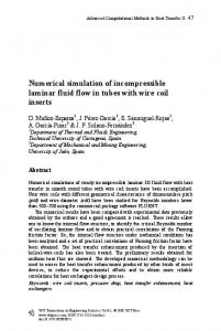
The present procedure for solving 3-D unsteady incompressible viscous flows has been applied to the flow around a 2-bladed SR7L propeller (Fig.1) at zero angle of attack. 50,000 of Reynolds number, 30.4~of blade pitch angle, and 0.881 of advance ratio. The advance ratio is defined as
where n is the number of propeller revolutions per second (rps) and D is the diameter of the propeller. Fig.2 shows isometric view of H-0 grid system for a 2-bladed SR7L propeller. Fig.3 shows the pressure coefficient distribution at several selected spanwise locations compared with experimental data by ~ushnell(~')and compressible Navier-Stokes equation solutions by Lim and sankar(ll). A fairly good agreement with experimental and other numerical data was achieved except near the leading edge region. This discrepancies of pressure distribution near the leading edge are attributable to the coarseness of grid near leading edge which precludes its ability to properly capture the strong leading edge vortex. The other possibilities of this discrepancy include uncertainties in the deflected blade shape and blade setting angle. Especially, experimental measurement of the blade setting angle is not sufficiently reliable. During wind tunnel tests at the Modane test facility, setting angle was adjusted to match power coefficient at different runs for the same flight conditions. Adjustment of as much as 2.6O were needed for some flight condition. The shift in pressure coefficient at root station (rW.284) may be due to the coarsely spaced grid near the leading edge of the nacelle. This d y spaced grid gives a cone shaped nose even though the actual nose is blunt. The conical flow characteristic is completely different to the flow ovex a blunt body. The comely spaced grid around a nacelle cannot also accurately compute the boundary layer on the nacelle and its interaction to the flow over blade, especially at inboard stations. Flow over a spinning propeller is rich in physical phenomena, and may be studied using scientific visualization tools. Fig.4 shows the pressure contours on the marine propeller surface and Fig.5 shows the spanwise distribution of aerodynamic force.. Fig.6 shows the simulated oil flow pattern. Significant outward flow on the solid surface are seen. This is due to the strong centrifugal forces acting on the very low speed flow (having low momentum) in the boundary layer. Fig.7 shows the streamlines over the blade of propeller. The formation of curved leading edge vortex and tip vortex are evident. The centrifugal pumping effects producing significant radial flow can not be produced h m inviscid analysis. The simulation also gives insight in the vortex formation over curved leading edge of the blade, although
additional changes to the grid are needed to resolve this vortex further. Fig.8 shows comparison of the convergence history of marine propeller problem without and with implementation of multigrid on the two grid system. Up to 30 50 % reduction in computer time was obtained using the multigrid technique. The CPU time is based on 25 iterations at each time step on the CRAY-YMP supercomputer on a 97x45~4 1 grid system. The surface pressure distributions are nearly the same as those of single grid system and are not plotted.
-
Conclusions An iterative time marching procedure for the solution of three-dimensional unsteady incompressible viscous flows has been applied to the flow around a marine propeller. The steady state solutions are obtained as asymptotic solutions of the time marching process. The present procedure is efficicntly solved by a pointimplicit method. This requires no matrix inversions, and is suitable for use on massively parallel machines. It was found that a multigridcoarse grid correction method(MGCGC) can be used to accelerate the convergence process. The propeller simulation gave generally good results compared with experiments and other numerical solutions. The curved leading edge vortex, tip vortex, and significant radial flow were captured by the present numerical simulation.
This work was sponsored by Office of Naval Research (ONR) under grant N00014-89-J-1319. The authors would like to appreciate Dr. S. G. Lekoudis and Dr. Edwin Rood, both of ONR, for their guidance and support of this work.
References Goldstein, S.,"On the Vortex Theory of Screw Propellers," Royal Society Proceeding, Vo1.123, no.792, pp.440-465, 1929. Sullivan, J. P.,"The Effect of Blade Sweep on Propeller Performance," AIAA Paper 77-176, 1977.
Downloaded by GEORGIA INST OF TECHNOLOGY on June 26, 2014 | http://arc.aiaa.org | DOI: 10.2514/6.1993-3503
Egolf, T. A., Anderson, 0.L., Edwards, D. E., and Landgrebe, A. J.,"An Analysis for High Speed Propeller-Nacelle Aerodynamic Performance; Vol.1. Theory and Initial Application and Vo1.2, User's Manual for the Computer Program," United Technologies Research Center, R79-912949-19, 1979. Jou, W. H.."Finite Volume Calculation of the Three Dimensional Flow Around a Propeller," AIAA Paper 82-0957.1982. Chaussee, D. S., Bober, L. J., and Kutler.,"Prediction of HIgh Speed Propeller Flow Fields Using a Three Dimensional Euler Analysis," AIAA Paper 83-0188, 1983. Bober, L. J., Yamamoto. 0..and Barton, J. M.,"Improved Euler Analysis of Advanced Turboprop Propeller Flow," AIAA Paper 861521,1986. Whitfield, D. L., Swafford, T. W., and Arnold, A. F. S.. and Belk, D. M.,"lhree Dimensional Euler Solution for Single Rotating and Counter Rotating Propfan," AIAA Paper 87-1197,1987. Srivastava. R. and Sankar, L. N.,"Application of an Efficient Hybrid Scheme for Aeroelastic Analysis of Advanced Propeller," AIAA Paper 900028. 1990. Matsuo, Y., Arakawa, C., Satio, S., and Kobayashi H.,"Navier-Stokes Computations for Flow Flied of an Advanced Turboprop," AIAA Paper 88-3094.1988. Hall, E. J., Delaney, R. A.. and Bettner, J. L.."Investigation of Advanced Counter Rotating Blade Configuration Concepts for High Speed Turboprop System ; Task 2, Unsteady Ducted Propfan Analysis," Final Report, NASA CR187106, 1991. Lim, T. B. and Sankar, L. N.,"Viscous Flow Computations of How Field around an Advanced Propeller," AIAA Paper 934873,1993. Roe, P. L.,"Approximate Riemann Solvers, Parameter Vectors and Difference Schemes." Journal of Computational Physics, Vol.43, 1981. pp.357-372. Kim, H. T.,"Computation of Viscous Flow Around a Propeller-Shaft Configuration with Infinite-Pitch Rectangular Blades." Ph.D. Thesis, The University of Iowa, Iowa City, IA, 1989. Patankar, S. V.,"A Calculation Procedure for TwoDimensional Elliptic Situations," Numerical Heat Transfer. Vol. 2. 1979. Sankar, L.N. and Park, W.G.,"An Iterative Time Marching Procedure f a Unsteady Viscous Flows," ASME-BED V01.20, pp. 281-284, 1991. Park. W. G.."A Three-Dimensional Multigrid Technique for Unsteady Incompressible Viscous Flows," Ph. D. Thesis, Georgia Institute of Technology, Atlanta, Georgia, March 1993.
Park, W. G. and Sankar, L. N.,"A Technique for the Prediction of Unsteady Incompressible Viscous Flows," AIAA Paper 93-3006, 1993. Viecelli. J. A.,"A Method for Inc!uding Arbitrary External Boundaries in the MAC Incompressible Fluid Computing Technique,"Journal of Computational Physics. Vol. 4, 1969, pp.543551. Leonard, B. P.,"A Stable and Accurate Convective Modelling Procedure Based on Quadratic Upstream Interpolation." Computer Methods in Applied Mechanics and Engineering, Vol. 19, 1979, pp.5998. Bushnell, P.,"Measurements of the Steady Surface Pressure Distribution on a Single Rotation Large Scale Advanced Numbers from 0.03 to 0.78," NASA CR 182124, 1988.
Fig. 1. Configuration of a marine propeller (%bladed SR7L)
44
0
02
0.4
0.0
0.8
I
1
Downloaded by GEORGIA INST OF TECHNOLOGY on June 26, 2014 | http://arc.aiaa.org | DOI: 10.2514/6.1993-3503
CHORD
44
0
02
0.4
0.8
CHORD
Fig.2.Body-fitted grid around a SR7L propeller
Fig.3. Surface pcsure disaibution at a selected SpanwiasEatians
0.8
I
1
Downloaded by GEORGIA INST OF TECHNOLOGY on June 26, 2014 | http://arc.aiaa.org | DOI: 10.2514/6.1993-3503
(ti) Drag distribution (Sectional)
dR
(c) Thrust distribution Elemental)
i-
k1 C
&
d
i
Q
&
&dR ~
b
&
&
(d) Torque disfl'bution (Elemental)
Fig5 S
m distribution of raodywnic fhcs
Fig.5. continued
Downloaded by GEORGIA INST OF TECHNOLOGY on June 26, 2014 | http://arc.aiaa.org | DOI: 10.2514/6.1993-3503
Fig.6.Simulated oil flow paaan on the blade surface
Fig-8.Comparisonof convergeom history with and without multigrid technique