May 25, 2004 - Kleinberg's HITS and Google's PageRank to assign authoritative weights ... In PageRank, a model of random walks is proposed such that.
Using a Layered Markov Model for Decentralized Web Ranking Jie Wu
Karl Aberer
August 19, 2004∗
EPFL Technical Report ID: IC/2004/70 School of Computer and Communication Sciences Swiss Federal Institute of Technology (EPF), Lausanne 1015 Lausanne, Switzerland {jie.wu, karl.aberer}@epfl.ch Abstract The link structure of the Web graph is used in algorithms such as Kleinberg’s HITS and Google’s PageRank to assign authoritative weights to Web pages and thus rank them. In HITS, a solid theoretical model is lacking and the algorithm often leads to non-unique or non-intuitive rankings where zero weights may inappropriately be assigned to parts of a network. In PageRank, a model of random walks is proposed such that the theory about the stationary state of a Markov process can be applied to assure convergence to a unique ranking. Both algorithms require a centralized computation of the ranking if used to rank the complete Web graph. In this paper, we propose a new approach based on a Layered Markov Model to distinguish transitions among Web sites and Web documents. Based on this model, we propose two different approaches for computation of ranking of Web documents, a centralized one and a decentralized one. Both produce a well-defined ranking for a given Web graph. We then formally prove that the two approaches are equivalent. This provides a theoretical foundation for decomposing link-based rank computation and makes the computation for a Web-scale graph feasible in a decentralized fashion, such as required for Web search engines having a peer-to-peer architecture. Furthermore, personalized rankings can be produced by adapting the computation at both the local layer and the global layer. Our empirical results show that the ranking generated by our model is qualitatively comparable to or even better than the ranking produced by PageRank.
Keywords: Web information retrieval, Web mining, link structure analysis, search engine, ranking algorithm, decentralized framework ∗ Written
on May 25, 2004.
1
1
Introduction
Applying the peer-to-peer architectural paradigm to Web search engines has recently become a subject of intensive research [6, 9, 12, 11]. Whereas for the decomposition of content-based retrieval techniques, such as classical text-based vector space retrieval or latent semantic indexing, various proposals have been made exploiting obvious possibilities of decomposition of the rank computation, for ranking methods based on the link structure of the Web it is much less clear of how to decompose their computation. We first briefly review the two most prominent link-based ranking algorithms - HITS [7] and PageRank [10], and then describe our main contribution towards enabling link-based ranking in peer-to-peer Web search engines.
1.1
Link-based Web Document Ranking
HITS has been introduced as a query-dependent approach, which first obtains a (small) subgraph of the Web relevant to a query result, which is obtained by using conventional retrieval techniques, and then applies the algorithm to this subgraph. On the other hand, PageRank is query-independent and operates on the whole Web graph directly. Disregarding this difference, both methods rely on the same principles of linear algebra to generate a ranking vector, by using a principal Eigenvector of a matrix generated from the (sub-)Web graph to be studied. It has been shown [5] that HITS is often instable such that the Eigenvectors returned by the algorithm depend on variations of the initial seed vector and that the resulting Eigenvectors inappropriately assign zero weights to parts of the graph. In short, HITS lacks strong theoretical basis assuring certain desirable properties of the resulting rankings. In PageRank the process of surfing the Web is used as intuitive model for assessing importance of Web pages and is modelled as a random walker on the Web graph. As the Web is not fully connected in practice, the process is complemented by random jumps such that transitions among non-connected pages are possible. The resulting transition matrix defines a stochastic process with a unique stationary distribution for the states, i.e. the Web pages, which is used to generate their ranking. The computation of PageRank (and similarly of HITS if it were applied to the complete Web graph) is performed on a matrix representation of the complete Web graph and inherently difficult to decompose as it would be required for a distributed computation in a peer-to-peer architecture.
1.2
Our Contribution
In this paper, we present a new model for Web link analysis with the goal of enabling decentralized rank computation. Different from the classic PageRank model where all states in the stochastic process are treated equally, the Layered Markov Model proposed by us exploits the inherent hierarchical structure and the self-similar character of the Web graph. In our Layered Markov Model the Web is no longer considered as a flat graph of Web documents, but characterized by a two-layer hierarchical structure: the graph of Web sites at the higher layer, and the graphs of Web documents at 2
the lower layer. A transition from one Web document to another is mapped to both transitions between Web sites at the higher layer and transitions between Web pages on the same Web site at the lower layer. We will show in this paper that this model has the following important properties: 1. We prove that the ranking method satisfies basic properties required for consistently producing rankings, similar as it has been done for PageRank. In particular, we show that the ranking is well-defined and produces a probability distribution over the Web documents. 2. We provide a Partition Theorem for Rank Computation showing that, using the model we can provide a distributed algorithm for computing the ranking that is equivalent to the canonical global algorithm. 3. Empirical experiments demonstrate that the ranking result produced by our approach is qualitatively comparable to or even better than that of PageRank. Link spamming is also defeated to a satisfiable degree. 4. While the model provides an alternative to existing link-based ranking methods allowing for distributed computation it also introduces the possibility to generate in an elegant way personalized rankings by including into the computational personal preferences at both the Web site layer and the Web page layer. This is particular interesting when used for the purpose of fighting link spamming.
2
Layered Markov Model
In this section, we first provide the problem definition for ranking Web documents. Then we summarize the classical PageRank algorithm. Finally we present our new Layered Markov Model for ranking Web documents.
2.1
The Ranking Problem
We first define the concept of ordered sets as they will be used in later definitions. Definition 1. A partially ordered set (poset) is a set X together with a relation ≤ such that for all a, b, c ∈ X: • a ≤ a (reflexivity) • a ≤ b, b ≤ c ⇒ a ≤ c (transitivity) • a ≤ b, b ≤ a ⇒ a = b (antisymmetry). A totally ordered set (toset) is a poset for which also for all a, b ∈ X: • either a ≤ b or b ≤ a. Definition 2. A ranking is a totally ordered set W bound to a set of Web objects O such that there exists a mapping rw : O → W. Then O is called a ranked Web object set. The particular element w ∈ W corresponding to a specific object o ∈ O is the ranking value of o, namely, rw(o) = w.
3
A ranking is often L1 -normalized such that the sum of all ranking values equals 1 and the result can be interpreted as a probability distribution. Definition 3. A document ranking is a ranking for Web documents. A site ranking is a ranking for Web sites. The problem of ranking Web documents is to find an algorithm to compute a document ranking for all documents in a given Web graph of pages. Ideally such an algorithm should be supported by an underlying model providing an interpretation of the result and the possibility to derive properties of the resulting rankings. Given the graph of Web pages GD (VD , ED ) with ND pages in total, we use the following notations: d ∈ VD is a Web page, hd is the number of links originating from page d, αd = h1d is the probability of a random surfer’s following one particular link from page d, hij is the number of links from page i to page j, pa(d) is the set of parent pages of d, i.e. those pages pointing to d, ch(d) is the set of child pages of d, i.e. those pages pointed to by d. In the classical PageRank model, a surfer is supposed to perform random walks on the flat graph generated by the Web pages, by either following hyperlinks on Web pages or jumping to a random page if no such link exists. A damping factor is defined to be the probability that a surfer does follow a hyperlink contained in the page where the surfer is currently located in. Suppose the damping factor is f , then the probability that the surfer performs a random jump is 1 − f . The classical PageRank Markov model is based on a square transition probability matrix M = {mij , i, j ∈ [1, ND ]}: αi ∗ hij hi 6= 0, dj ∈ ch(di ) 0 hi 6= 0, dj ∈ / ch(di ) mij = (1) 1 h = 0 i ND However, this matrix does not ensure the existence of the stationary vector of the Markov chain which characterizes the surfer behavior, i.e., the PageRank vector. As widely accepted, the unaltered Web creates a reducible Markov chain. Thus, the PageRank algorithm enforces a so-called maximal irreducibility adjustment to make a new irreducible transition matrix: ˆ = f M + 1 − f ee0 M ND
(2)
ˆ is the where e is the column vector of all 1s and e0 is e’s transposed. M primitive, thus the power method will finally produce the stationary PageRank vector. In other informal words, the application of PageRank algorithm over a given square matrix is equivalent to first applying the maximal irreducibility adjustment to the matrix, then applying the power method to the new matrix in order to obtain its principal Eigenvector. ˆ (G) to denote the function of generating such We also use M (G) and M ˆ (G), matrices for a given graph G. Remember that in the function body of M personalization of rankings can be obtained by replacing e with a personalized distribution vector in equation (2).
4
2.2
Why Layered Markov Model
While PageRank assumes that the Web is a flat graph of documents and the surfers move among them without exploiting the hierarchical structure, we consider the Layered Markov Model as a suitable replacement for the flat Markov chain to analyze the Web link structure for the following reasons: • The logical structure of the Web graph is inherently hierarchical. No matter, whether the Web pages are grouped by Internet domain names, by geographical distribution, or by Web sites, the resulting organization is hierarchical. Such a hierarchical structure does definitely influence the patterns of user behavior. • Web is shown to be self-similar [4] in the sense that interestingly, part of it demonstrates properties similar to those of the whole Web. Thus instead of obtaining a snapshot of the whole Web graph, introducing substantial latency, and performing costly computations on it, bottom-up approaches, which deal only with part of the Web graph and then integrate the partial results in a decentralized way to obtain the final result, seem to be a very promising and scalable alternative for approaching such a large-scale problem.
Figure 1: Phases and sub-states in Layered Markov Model. Figure 1 illustrates a Layered Markov Model structure. The model consists of 12 sub-states (small circles) and 3 super-states (big circles), which are referred to as phases in [2]. There exists a transition process at the upper layer among phases and there are three independent transition processes happening among the sub-states belonging to the three super-states.1 1 Please note the figures of layered models here are only for the purpose of illustration, and the transition probabilities in the matrices used in our examples later are not necessarily
5
When applying the Web surfer paradigm, a phase could be considered as a surfer’s staying within a specific Web site or a particular group of Web pages. The transition among phases corresponds to a surfer’s moving from one Web site or group to another. The transition among sub-states corresponds to a surfer’s movement within the site or group. Thus a comprehensive transition model should be a function of both the transitions among phases and the transitions among sub-states. In other words, the global system behavior emerges from the behaviors of decentralized and cooperative local sub-systems. We consider a two-layer model in the following to keep explanations simple, but the analysis can be extended to multi-layer models using similar reasoning. We introduce now the notations to describe the two-layer model. • Given the number of phases NP , we use {1, 2, · · · , NP } to label the individual phases and denote the phase active at time t as a variable Z(t). The set of phases is denoted by P = {P1 , P2 , · · · , PNP }. • For each phase PI the number of its sub-states is nI . We use {1, 2, · · · , nI } to label the individual sub-states and denote the state at time t as a variable z I (t). The set of sub-states of phase PI is denoted by OI = {oI1 , oI2 , · · · , oInI }. The overall set of sets of sub-state is denoted by O = {O1 , O2 , · · · , ONP }. • The transition probability at the phase layer is given by Y = {yIJ } where yIJ = P (Z(t + 1) = J|Z(t) = I) and 1 ≤ I, J ≤ NP . The initial state distribution vector is denoted by vY . • For each phase I, the transition probability at the sub-state layer is given by UI = {uIij } where uIij = P (Z(t + 1) = I, z I (t + 1) = j|Z(t) = I, z I (t) = i) and 1 ≤ i, j ≤ nI . In addition, U is defined to be the set of all substate transition matrices: U = {U1 , U2 , · · · , UNP }. There exists a one-toone mapping between P and U, namely each phase PI has its sub-state transition matrix U I , 1 ≤ I ≤ NP . The set of initial state distribution NP 1 2 vectors is denoted by vU = {vU , vU , · · · , vU }. When context is clear, we also use the index of a phase or a sub-state to designate the phase or sub-state. For example, phase 2 for P2 and its sub-state 3 for o23 in O2 . An overall system state is denoted by a (phase,sub-state) pair like (2,3) which means the system is at the sub-state 3 of phase 2. In addition, PNP NP = I=1 nI is used to denote the total number of overall system states. An overall system state is also called a global system state in contrast to a local sub-state (i.e. a sub-state local to a phase). Definition 4. A (two-layer) Layered Markov Model is a 6-tuple LMM = (P, Y, vY , O, U, vU ) where each dimension has the meaning explained above.
2.3
LMM for Ranking Global System States
We want to use the Layered Markov Model to compute a ranking for all global system states, i.e., a stationary (if possible) distribution vector for all global system states. Such a ranking also should be uniquely defined. related to the edges of the graph shown in this figure.
6
We assume that state transition between two global system states is always abstracted as first an inter-phase transition, and then an intra-phase transition. As an example, suppose we have a phase transition matrix Y, and three sub-state transition matrices U1 of the four-sub-state phase I, U2 of the threesub-state phase II, and U3 of the five-sub-state phase III as follows: .3 .3 .2 .2 .1 .3 .6 .5 .1 .1 .3 Y = .2 .4 .4 U1 = .1 .2 .6 .1 .3 .5 .2 .4 .3 .1 .2 .6 .02 .2 .1 .08 .05 .2 .5 .05 .2 .2 .1 .7 2 3 .1 .8 .1 U = .1 .2 U = .4 .1 .2 .7 .1 .05 .1 .05 .05 .05 .9 .5 .2 .1 .1 .1 We want to rank the 12 global system states according to the general authority implied by the transition link structure. To do so, we need to obtain a global transition probability matrix for the 12 global system states. For Layered Markov Models with homogeneously structured sub-states, i.e. all subgraphs corresponding to phases have the same structure, the global transition matrix can be obtained conveniently as a matrix tensor product [15]. Unfortunately, it’s impossible to do so for non-homogeneous sub-states as they occur for any practical Web graph. Instead we will derive such a matrix relying our notion of layer-decomposability.
2.3.1
Layer-Decomposability
Informally, the property of layer-decomposability ensures the legitimacy of decomposing the transition between two global system states to the two steps of first inter-phase transition then intra-phase transition. In order to define the decomposability between layers, we first introduce the concept of gatekeeper sub-state. Definition 5. A gatekeeper sub-state oIG of a phase PI is a virtual sub-state appended to the phase, such that it connects to every other sub-state and every other sub-state is connected to it. After the introduction of gatekeeper sub-states for phases, the decomposability of a Layered Markov Model is defined as below. Definition 6. Layers in a Layered Markov Model are decomposable if the transition probability between two given non-gatekeeper sub-states in their two corresponding phases satisfies: P (Z(t + 1) = J, z(t + 1) = j|Z(t) = I, z(t) = i) =
J
J
P (Z(t + 1) = J|Z(t) = I)P (z (t + 1) = j|z (t) =
(3) oJG )
The definition basically assures in the model that whenever a phase transition takes place, it has to go through the gatekeeper sub-state of the destination phase. The gatekeeper sub-state functions as the boundary between inter-phase transitions and intra-phase transitions. 7
Denoting the transition probability in phase PJ from the gatekeeper substate oJG to sub-state oJj by uJGj , the elements of the resulting global transition matrix W are computed as follows: w(I,i)(J,j) = yIJ uJGj
(4)
We show that Lemma 1. The resulting transition matrix W satisfies the Markovian property. Proof. For each J ∈ [1, NP ], we have X uJGj = 1
(5)
j
since this is the sum of the transition probabilities from the gatekeeper sub-state oJG to all the sub-states oJj , j = 1, 2, · · · , nJ within phase PJ . Thus given an overall system state (I, i), XX X XX X w(I,i)(J,j) = yIJ uJGj = yIJ uJGj = 1 J
2.3.2
j
J
j
J
j
Transition Probabilities of Gatekeeper Sub-states
To compute (4), for each phase J we have to obtain the uJGj values of all j ∈ [1, nJ ]. We already have the Markovian (not necessarily irreducible) transition matrix UJ . After adding the new virtual gatekeeper sub-state, we need to make ˆ J Markovian as well. A possible method the new (nJ + 1) × (nJ + 1) matrix U of applying such a change is: · ¸ αUJ (1 − α)e ˆJ = U J T (vU ) 0 where 0 < α < 1 is an adjustable parameter, e is the column vector of all 1s J and vU is the initial state distribution vector for all the non-gatekeeper substates within PJ , as we have described before. The new matrix UˆJ is not only Markovian, but also irreducible and primitive. This method is actually known as the approach of minimal irreducibility in the context of PageRank computation. In detail, applying the power method on UˆJ will eventually produce its principal Eigenvector. After that, the last element of the vector, which corresponds to the appended gatekeeper sub-state in our case, is removed and the remaining nJ elements are re-normalized to J make the sum up to 1. The resulting vector πU is considered as the stationary distribution over all the non-gatekeeper sub-states within the given phase J. J We take the nJ elements of the stationary distribution vector πU as the values J of all uGj , j ∈ [1, nJ ]. Interestingly enough, it is shown in [8] that this method is equivalent in theory and in computational efficiency to Google’s method of maximal irreducibility. Thus, given the adjustable factor α, we actually take the PageRank values of the local sub-states of PJ as their uJGj values, j ∈ [1, nJ ]. To compute a ranking for the system states, we need to ensure the primitivity of the new global transition matrix. 8
Lemma 2. If Y is primitive and the PageRank values of the local sub-states of PJ are taken as their uJGj values, j ∈ [1, nJ ], the global transition matrix W is also primitive. Proof. This is a natural consequence of all the uJGj values’ being positive. Thus W has only one Eigenvalue on its spectral circle. The corresponding Eigenvector could be used to rank the states in the overall system. However, we do not make the assumption in our analysis that both Y and U are primitive, we are only sure that both of them are Markovian. Even if they are not primitive, we can make the resulting W primitive by adopting the same approach as taken in PageRank, the so-called method of maximal irreducibility, by connecting every pair of nodes via random jumps. Once the primitivity is achieved, we can always compute the ranking of the system states. We now compute the W for our example given by the four Markovian matrices Y, U1 , U2 and U3 . First, we compute the PageRank vectors for three J phases (denoted by πG ,J = 1, 2, 3 here): 0.4557 0.3054 0.1038 0.1191 0.2312 2 1 π = 0.2691 π 3 = 0.2014 πG = G 0.2582 G 0.1106 0.6117 0.2052 0.1285 Then we use the equation (4) to obtain the new W: 0.0305 0.0231 0.0258 0.0205 0.0357 0.0305 0.0231 0.0258 0.0205 0.0357 0.0305 0.0231 0.0258 0.0205 0.0357 0.0305 0.0231 0.0258 0.0205 0.0357 0.0611 0.0462 0.0516 0.0410 0.0477 0.0611 0.0462 0.0516 0.0410 0.0477 W= 0.0611 0.0462 0.0516 0.0410 0.0477 0.0916 0.0694 0.0775 0.0616 0.0596 0.0916 0.0694 0.0775 0.0616 0.0596 0.0916 0.0694 0.0775 0.0616 0.0596 0.0916 0.0694 0.0775 0.0616 0.0596 0.0916 0.0694 0.0775 0.0616 0.0596 0.1835 0.1835 0.1835 0.1835 0.2447 0.2447 0.2447 0.3059 0.3059 0.3059 0.3059 0.3059
0.2734 0.2734 0.2734 0.2734 0.1823 0.1823 0.1823 0.0911 0.0911 0.0911 0.0911 0.0911
0.0623 0.0623 0.0623 0.0623 0.0415 0.0415 0.0415 0.0208 0.0208 0.0208 0.0208 0.0208
0.1209 0.1209 0.1209 0.1209 0.0806 0.0806 0.0806 0.0403 0.0403 0.0403 0.0403 0.0403 9
0.0664 0.0664 0.0664 0.0664 0.0442 0.0442 0.0442 0.0221 0.0221 0.0221 0.0221 0.0221
0.0807 0.0807 0.0807 0.0807 0.1077 0.1077 0.1077 0.1346 0.1346 0.1346 0.1346 0.1346
0.0771 0.0771 0.0771 0.0771 0.0514 0.0514 0.0514 0.0257 0.0257 0.0257 0.0257 0.0257
(6)
0.0658 5 0.0682 5 1 : (1, 1) 0.0498 7 0.0547 7 2 : (1, 2) 0.0556 6 0.0596 6 3 : (1, 3) 0.0442 10 0.0499 10 4 : (1, 4) 0.0495 8 0.0545 8 5 : (2, 1) 0.1118 3 0.1073 3 6 : (2, 2) π ˜W = πW = 7 : (2, 3) 0.2541 1 0.2281 1 0.1683 2 0.1562 2 8 : (3, 1) 0.0383 12 0.0452 12 9 : (3, 2) 0.0744 4 0.0760 4 10 : (3, 3) 0.0408 11 0.0474 11 11 : (3, 4) 0.0474 9 0.0530 9 12 : (3, 5) Figure 2: Ranking results of Approach 1 & 2 The elements of this global system transition matrix are the probabilities of transitions among global system states. The elements of both the rows and columns are in the order of (1,1), (1,2), (1,3), (1,4), (2,1), (2,2), (2,3), (3,1), (3,2), (3,3), (3,4), (3,5). 1 · · · 12 are assigned as their corresponding global system state index. For example, the element w(12)(7) = w(3,5)(2,3) is the transition probability from the sub-state 5 of phase 3 (global system state 12) to the substate 3 of phase 2 (global system state 7). Layer decomposability assures that w(3,5)(2,3) = y32 u2G3 = 0.5 × 0.6117 = 0.3059. As equation (4) does not depend on i anymore given a global system state (I, i), we can find that in the matrix W rows pertaining to a particular value I are constant. At this point, we are able to compute a ranking for the global system states. There are two possible approaches. Approach 1: We apply the standard PageRank algorithm to W to rank all states, i.e. we apply the method of maximal irreducibility to W before we launch the power method to compute the principal Eigenvector. We obtain πW as follows: The first column in Figure 2 above is the list of global system states with there index number on the left-hand side. The middle vector πW gives the rank values (PageRank values) we computed based on the transition matrix W , and the column neighboring to the vector on the right-hand side gives the order numbers of the states ranked by their rank values. Approach 2: On the other hand, as Y is already primitive, hence W is primitive as well. We can compute directly its stationary state distribution without applying the Google’s maximal irreducibility method. The resulting ranking is shown by the right vector π ˜W in Figure 2. We can see, other than minor differences in the absolute values, the two results rank all system states in an identical order. The results imply that, in the Layered Markov Model defined by Y, U1 , U2 and U3 , the top three (highly ranked) overall system states are number 7, 8 and 6, namely (2,3), (3,1) and (2,2). As in both Approach 1 and Approach 2, we have to compute in advance the global transition matrix W in order to derive the ranking of the global system states, we consider these two as centralized approaches for computing 10
the global system state ranking. The differences between them are summarized in the following table where Pri. stands for Primitivity and MI stands for the Maximal Irreducibility trick used in PageRank: Approach 1 2
Pri. of Y Yes or No Yes
Pri. of W Yes or No Yes
If MI for W Yes No
Table 1: Differences between Approach 1 and 2
2.3.3
Partition Theorem for Rank Computation
A natural question is now that given the PageRank ranking for all four matrices, Y, U1 , U2 and U3 , is it possible to obtain the stationary distribution for the global system states without deriving a new matrix W and applying the PageRank algorithm to it? We introduce now such an algorithm step-by-step: 1. At the phase level, if Y is already primitive, we can compute its stationary distribution π ˜Y without applying the maximal irreducibility method to Y before the power method is applied. The element for phase I in the distribution vector is denoted by π ˜Y (I). Certainly, we can also compute the slightly different πY by applying the maximal irreducibility method to Y even if Y is already primitive. We will see later on why we don’t make this choice. 2. At the sub-state level within phases, for each phase I, we compute its I stationary distribution πG by applying the PageRank algorithm to UI . Remember this resulting vector is related to our introduced gatekeeper sub-state of each phase PI . We denote the element for sub-state i in the I distribution vector by πG (i). 3. For each global system state (I, i), we assign it a value as follows: I π ˜ (I, i) = π ˜Y (I)πG (i)
(7)
The assignments to all global system states form a state distribution π. We call this the Layered Method of rank computation. The result of this computation has the following (expected) property. Theorem 1. The resulting vector of the Layered Method of rank computation is a probability distribution. Proof. XX I
i
π ˜ (I, i) =
XX I
I π ˜Y (I)πG (i) =
i
X I
11
π ˜Y (I)
X i
I πG (i) = 1
We give an example illustrating the computation: we want to compute the ranking value assigned to the global system state 7 : (2, 3). Approach 3: The PageRank vector πY for Y is: πY = (0.2315, 0.4015, 0.3670)T We can replace π ˜Y (I) in (7) with πY (I) and the result is still a probability distribution. The corresponding multiplication becomes: 2 π(2, 3) = πY (2)πG (3) = 0.4015 × 0.6117 = 0.2456
Unsurprisingly, this value is different from πW (2, 3) that we’ve computed before. Approach 4 (the Layered Method): The vector π ˜Y for Y is: π ˜Y = (0.2154, 0.4154, 0.3692)T Thus:
2 π ˜ (2, 3) = π ˜Y (2)πG (3) = 0.4154 × 0.6117 = 0.2541
Notice that this value is equal to that of π ˜W (2, 3) we have obtained previously. We call Approach 3 and Approach 4 the decentralized approaches for computing the global system state ranking, as we do NOT have to compute in advance the global transition matrix W. Instead we compute the ranking for the phases (or Web sites for the case of Web document ranking), the individual rankings for the sub-states in each phase (or the individual Web document rankings for each Web site), which can be done in a parallel or decentralized fashion. The differences between Approach 3 and 4 are summarized in the table below: Approach 3 4
Pri. of Y Yes or No Yes
If MI for Y Yes No
Table 2: Differences between Approach 3 and 4 Now we want to show the equality of the values obtained from Approach 2 and Approach 4 in the example is not accidental. Corollary 1. Approach 2 and Approach 4 (the Layered Method) are equivalent. This corollary results from the following theorem. Theorem 2. Give LMM = (P, Y, vY , O, U, vU ) as a Layered Markov Model where Y is primitive. The following vectors are first computed: the stationary I state distribution vector π ˜Y of Y, the PageRank vectors πG , I ∈ [1, NP ]. A new matrix W and a new vector π ˜ are derived in the following fashion: PNP ˜ are NP = I=1 nI , i.e., the total 1. Both the size of W and the length of π number of the global system states in the model LMM. Every element of W and every element of π ˜ correspond to a global system state (I, i) ordered by I ∈ [1, NP ] and i ∈ [1, nI ]. J (j). 2. Every element of W is defined by w(I,i)(J,j) = yIJ πG
12
I 3. Every element of π ˜ is defined by π ˜ (I, i) = π ˜Y (I)πG (i).
Then W is also primitive and its stationary state distribution vector is exactly π ˜. Proof. For a primitive matrix, we know its stationary state distribution vector is the principal Eigenvector of its transposed matrix. Lemma 2 assures that W is primitive. Lemma 1 says W is Markovian, thus the principal Eigenvalue of W is 1. Then it remains to show W0 π ˜=π ˜ which is equivalent to that, given (I, i), P P ˜ (J, j) = π ˜ (I, i) J j w(J,j)(I,i) π P P I J I πY (J)πG (j) = π ˜Y (I)πG (i) ⇔ J j yJI πG (i)˜ P P J I I ⇔ πG (i) J yJI π ˜Y (J) j πG (j) = π ˜Y (I)πG (i) P I I ˜Y (J) = π ˜Y (I)πG (i) ⇔ πG (i) J yJI π P ˜Y (J) = π ˜Y (I) ⇔ J yJI π The last equality is guaranteed by the fact that π ˜Y is the stationary state distribution vector of Y. We call Theorem 2 the Partition Theorem for Rank Computation as the rank computation for the global system states in a Layered Markov Model can be decomposed into several steps that can be performed in a decentralized or/and parallel fashion, if decomposability is assumed and the phase transition matrix is primitive. The computation proceeds as follows: • At the phase layer, computation of the stationary distribution for the phase transition matrix. • At the sub-state layer, computation of the PageRank for individual substate stationary distribution for the sub-state transition matrix. • The aggregation of those vectors where only O(NP ) multiplications are necessary. In contrast, previous methods require to do a large number of multiplications of two NP × NP matrices until the resulting vector converges.
3
Application to Web Information Retrieval
We now discuss how the theoretical results obtained can be applied in the context of Web Information Retrieval. We know that search engines take into consideration both query-based ranking (for example, distances between queries and documents based on the Vector Space Model) and link-structure-based ranking (typically PageRank in Google and HITS-derived algorithm in Teoma) when ordering search results. We focus on the second aspect.
13
3.1
Different Abstractions for the Web Graph
Previous research work focused on the page granularity of the Web, i.e., a graph where the vertices are Web pages and the edges are links among pages. We propose to model the Web graph at the granularity of Web site. We call the graph at the document level the DocGraph, and the graph at the Web site level the SiteGraph. We also use the notion of SiteLink to designate hyperlinks among Web sites and DocLink for those among Web documents. Thus, the graph of Web documents GD (VD , ED ) with ND pages is a in a DocGraph. We assume its corresponding SiteGraph is GS (VS , ES ) with NS Web sites in total, a vs ∈ VS is a Web site, an es ∈ ES is a SiteLink. We use the notations GD (VD , ED ), vd , ed for a DocGraph. We also use the shorthand d and s to represent a Web document and a Web site respectively. Taking one page d, we denote its corresponding site as s = site(d) with ns = size(s) local Web documents in total. Vd (s) ⊆ VD is the set of all local Web pages of the particular Web site s. Ed (s) ⊆ ED is defined to be the set of those ed whose both originating and destination documents are members of Vd (s). Gsd = (Vd (s), Ed (s)) is defined to be the subgraph restricted with the Web site s. We call the ranking of Web sites the SiteRank for the SiteGraph and the ranking of Web documents the DocRank for the DocGraph. PageRank is an example of DocRank, but DocRank can be computed in a way other than PageRank, for example, as in our approach in a decentralized fashion. We also use the notions SiteRank(GS ) and DocRank(GD ) to refer to the SiteRank result of GS and DocRank result of GD respectively. When we are using the maˆ S of GS and M ˆ D of GD , we also use SiteRank(M ˆ S ) and trix representations M ˆ DocRank(MD ) to denote the rankings. The SiteGraph was studied in earlier work [3] under the name of hostgraph for purposes other than rank computation. This provided several good arguments on why the abstraction at the site level is useful. However, it is worth noticing that our notion of SiteGraph allows for the derivation of a dynamic or virtual graph of Web sites when we use dynamic or virtual relationships among Web pages instead of the static Web links. For example, when we use statistical information on navigation obtained from Web client traces, which are normally very different from the static Web link structure, as the set of edges E, we obtain a Web client trace-based SiteGraph. Similarly, a DocGraph using client traces can be defined. Early foundation work on such methods was presented in [13]. Thus hostgraph is simply one special type of SiteGraphs which uses the static hyper links among Web pages to define the edges.
3.2
Layered Method for DocRank
Having the analytical results above, we compute the DocRank for a given Web graph in the following steps: 1. Derive the global DocGraph GD (VD , ED ) from the given Web graph. Typically, DocLinks are processed. 2. Derive the global SiteGraph GS (VS , ES ) from the DocGraph. Nodes in the SiteGraph are the Web sites. Edges are grouped together according to Web sites. The numbers of SiteLinks are counted. 14
3. For each Web site s, derive the subgraph Gsd , its matrix representation ˆs =M ˆ s ) using the classical ˆ (Gs ) and compute its πD (s) =DocRank(M M d d d PageRank algorithm. This step can be completely decentralized in a peerto-peer search system. 4. For the global SiteGraph GS (VS , ES ), we first derive a primitive transition matrix and then compute its principal Eigenvector. The primitivity of the transition probability matrix is required by Theorem 2. In practice, we ˆS =M ˆ (GS ) which is primitive and its principal Eigenvector compute M πS = (πS (s1 ), · · · , πS (sNS ))0 as the SiteRank. 5. For i = 1, · · · , NS , we list the ND DocRank vectors πD (si ) and create an aggregate vector from them: 0
0
πD = (πD (s1 ) , · · · , πD (sNS ) )0 By applying Theorem 2, we perform a weighted product to obtain the final global ranking for all documents in the DocGraph GD (VD , ED ): 0
0
DocRank(GD ) = (πS (s1 )πD (s1 ) , · · · , πS (sNS )πD (sNS ) )0 Personalization of rankings can be easily implemented in our layered method for DocRank. Personalization at the lower layer, i.e., the layer of local Web documents within specific Web sites, can be realized in Step 3 by providing different ˆ (Gs ). Similarly, personalization personalized vectors in the function body of M d at the higher layer, i.e., the layer of Web sites, can be realized in Step 4. Of course, personalization at both layers can be combined to use together.
3.3
Empirical Results
We made some initial experiments on a recently crawled snapshot of our campus Web. We started from the home page of the university, www.epfl.ch, and let the crawler follow the hyperlinks and retrieve Web pages. Different from many other previous published experiments, we did not exclude dynamic Web pages generated by server-side scripts. The reason is that nowadays most Web sites use them as a powerful vehicle to provide dynamic and fresh information. Without including them, the captured Web graph would be a rather skewed one. However, crawling dynamic pages often causes infinite loop for all kinds of possibilities. To avoid this, researchers usually let the crawler fly and then stop it after it has been running for a period of time. Our partial Campus Web graph was captured in late 2003. In this graph there are 218 Web sites and 433707 Web pages altogether. We follow the steps described in Section 3.2 to compute the SiteRank of the SiteGraph of this partial Campus Web, the DocRanks of every Web site, and finally the global DocRank for all Web pages in this partial Campus Web. The result is presented in Figure 4. To make comparison, we also apply the classical PageRank algorithm to the set of all Web pages to obtain the PageRank for them. The result is presented in Figure 3. The left columns are the lists of the document identifiers with their corresponding URLs in the right columns. Documents are listed in an descending order of the computed rank values. In both figures we only present the top 15 entries of both rankings. The main reason is that Internet searchers tend to only care about the top ranked 15
16 1737 73612 73613 73614 18282 677 570 459683 73635 73636 73637 122990 90330 614
http://www.epfl.ch/ http://research.epfl.ch/ http://research.epfl.ch/research/Webdriver?LO=... http://research.epfl.ch/research/Webdriver?MIval=... http://research.epfl.ch/research/Webdriver?LO=... http://research.epfl.ch/research/Webdriver?MIval=... http://www.epfl.ch/place.html http://www.epfl.ch/styles/dynastyle.php http://dmawww.epfl.ch/roso.mosaic/ismp97/... http://research.epfl.ch/research/Webdriver?LO=... http://research.epfl.ch/research/Webdriver?MIval=... http://research.epfl.ch/research/Webdriver?LO=... http://lamp.epfl.ch/˜linuxsoft/java/jdk1.4/docs/... http://lampwww.epfl.ch/˜linuxsoft/java/jdk1.4/docs/... http://sti.epfl.ch/
Figure 3: Ranking result given by PageRank search results. Limit of space is another reason. Since some URLs are too long, we put the suspension points at the end of them and cut the actual remaining substrings which may well take another 100 characters. We find very interesting that, in Figure 3, the top entries of the PageRank result are dominated by some pages which share an identical URL prefix. Further investigation shows that all of them have a huge in-degree number. For example, the dynamic page 73612 has 17004 incoming links and most of its originating pages have the same URL prefix http://research.epfl.ch/research/Webdriver? which means they are generated by the same server-side script and heavily linked among each other. Similarly, the static page 122990 has 6425 incoming links and most of its originating pages have as well the same URL prefix http://lamp.epfl.ch/~linuxsoft/java/jdk1.4/docs/ which means they are all javadocs of jdk1.4 and also heavily linked among each other. A side note is that page 122990 and 90330 are actually an identical one, since lamp.epfl.ch and lampwww.epfl.ch are two different host names of one Web server. Hence they have almost identical rank values. It seems that the agglomerate structure of these document collections boosts drastically their PageRank values and this fact has been widely used by PageRank spammers such that even a new business has been created to make the most of PageRank. On the other hand, the ranking result computed by our Layered Method based on LMM gives a very neat list of entries which really cover many authoritative aspects of the university, such as central place (677), student bar (73324), student organization (153), 150 anniversary page (572), faculty of engineering (2884), search (73446), news (678), internal journal (71973 and 71975), press information (681), vice presidency of education (71961), etc.. In the Layered Method, the role played by the entangled cross links has been made much less important due to the effect of introducing the SiteRank of 16
16 570 677 73324 2196 153 572 2884 73446 678 581517 71973 71975 681 71961
http://www.epfl.ch/ http://www.epfl.ch/styles/dynastyle.php http://www.epfl.ch/place.html http://satellite.epfl.ch/ http://lcsmwww.epfl.ch/ http://cssa.epfl.ch/ http://www.epfl.ch/150/ http://sti.epfl.ch/news/AG/AG-Faculte-STI08.html http://mysearch.epfl.ch/help/?la=fr http://www.epfl.ch/niceberg/content/1/ http://smte.epfl.ch/francais/impressum.php http://spi.epfl.ch/Jahia/site/spi/cache/offonce/pid/... http://spi.epfl.ch/page33282.html http://www.epfl.ch/impressum.html http://vpf.epfl.ch/
Figure 4: Ranking result given by our Layered Method based on LMM the owner Web site as a crucial part of the final global ranking for a particular Web page. It shows that the global page ranking algorithm is not necessarily the best possible ranking method. We actually have obtained substantial qualitative improvements by using our Layered Method for ranking. It demonstrates the capability of the LMM model to defeat link spamming to a very satisfiable degree by making use of information implied in the inherent hierarchical structure of the Web.
4
Related Work
When considering a peer-to-peer architecture the strategy for computing SiteRank and DocRank need to be considered. In a flat peer-to-peer architecture SiteRank could be a shared resource among all peers, i.e. globally available, which is realistic as its value changes less rapidly. DocRank computations are performed by individual peers, which would ideally map to Web servers. This would in particular open the possibility to obtain access to the hidden Web. Alternatively, super-peer architectures can be considered, where rank aggregation is only performed at super-peers and individual peers provide their local DocRanks. Hierarchical Hidden Markov Models are used in [2] and similar work to determine optimal parameters for a Hidden Markov Model given observed outputs from the hidden states. The main purpose of this work is to reduce the complexity of learning a hidden model for large-scale and highly complex application domains, such as analysis of traffic data from ISDN traffic, Ethernet LAN’s, Common Channel Signaling Network (CCNS) and Variable Bit Rate (VBR) video, etc.. For such problems, applying the standard HMM learning algorithm does not generate an acceptable results as studies have shown. The study in this paper is fundamentally different from this work both in the model and the problem itself: In our model, we do not have observed outputs while a hidden model has. The purpose is also different. We do not aim at learning system parameters, but to mine the link structure and obtain a ranking
17
for all global system states. Most Web rank computation algorithms are developed based on PageRank or HITS, both of which consider a flat Web graph. Due to the huge-scale of the Web, such algorithms have inherent bottlenecks in scalability, cost of computation, latency, etc. since they can only be done in a centralized way. While many research groups are working on how to optimize the existing PageRank, HITS and their derived algorithms, little progress has been made in how to compute Web rankings in a decentralized fashion. We investigate this problem and devise two directions to realize decentralized computation of Web rankings: 1. Algebraic approach. We allow different semantic rankings being computed for the same subgraph in a parallel or decentralized fashion. The final ranking result is obtained by algebraic combination of weighted semantic rankings for subgraphs. Algebraic operations such as contraction and folding are defined to aggregate ranking vectors obtained with different granularity. More details on this approach are found in [14] and [1]. 2. Modelling approach. The work presented in this paper goes in this direction by proposing a new Layered Markov Model to model the surfing activities in the Web. We establish a strict analytical model and give the corresponding algorithm based on the theoretical result. The algorithm takes advantage of the hierarchical structure of the Web and successfully decomposes the rank computation at the Web scale into parallel or distributed tasks. In addition, the algorithm also leaves room for personalization of Web rankings.
5
Conclusion and Future Work
In this paper, we introduce a novel link-structure analysis method based on a Layered Markov Model. Our model differs substantially from the classic rank computation models that consider a flat Web graph. Our layered model makes use of the inherent hierarchical logical structure of the Web and the self-similar character of the Internet. We provide a strict analysis of our model for the Web ranking problem and give the Partition Theorem for Rank Computation. Such a formal result backs up theoretically the rank computation of the Internet-scale Web graph in a completely distributed way. This removes the radical obstacle and limitation that the existing rank computation algorithms have to suffer in terms of requiring global computation. In addition, our model also makes it easy to personalize rankings at both the higher Web site layer and the lower Web page layer. Empirical experiments give good results and show that link spamming which has been a headache for some global ranking algorithm is also nicely defeated to a very satisfiable degree. In the future, we plan to continue extensive experiments to empirically compare the ranking results produced by representative algorithms and our layered algorithm. The comparison between this modelling approach and our algebraic approach will be made as well. In addition to the comparison of ranking results, performance and resource usage of the algorithms, which are also critical
18
to search engines, will be studied. Work of combining query-based ranking and link-based ranking will also be carried out. Disclaimer We acknowledge that PageRank is just one of many criteria, measures and tools that Google uses to rank search results for users. We only focus on the technical issues of link-based ranking algorithms. This paper, in no way, speaks for or against Google.
References [1] Karl Aberer and Jie Wu. A framework for decentralized ranking in web information retrieval. In Web Technologies and Applications: Proceedings of 5th Asia-Pacific Web Conference, APWeb 2003, volume LNCS 2642, pages 213–226, Xi’an, China, April 2003. Springer-Verlag. [2] Jafar Adibi and Wei-Min Shen. Self-similar layered hidden Markov models. Lecture Notes in Computer Science, 2168:1–15, 2001. [3] Krishna Bharat, Bay-Wei Chang, Monika Henzinger, and Matthias Ruhl. Who links to whom: Mining linkage between web sites. In Proceedings of the IEEE International Conference on Data Mining (ICDM ’01), San Jose, USA, November 2001. [4] Stephen Dill, S. Ravi Kumar, Kevin S. McCurley, Sridhar Rajagopalan, D. Sivakumar, and Andrew Tomkins. Self-similarity in the web. In The VLDB Journal, pages 69–78, 2001. [5] A. Farahat, T. LoFaro, J. C. Miller, G. Rae, and L. A. Ward. Existence and Uniqueness of Ranking Vectors for Linear Link Analysis Algorithms. SIAM Journal on Scientific Computing, (submitted), 2003. [6] Omprakash D Gnawali. A keyword-set search system for peer-to-peer networks. Master’s thesis, Department of Electrical Engineering and Computer Science, MIT, May 2002. [7] Jon Kleinberg. Authoritative sources in a hyperlinked environment. In Proceedings of the ACM-SIAM Symposium on Discrete Algorithms, 1998. [8] Amy N. Langville and Carl D. Meyer. Deeper inside pagerank. Internet Mathematics, February 2004. [9] Jinyang Li, Boon Thau Loo, Joseph M. Hellerstein, M. Frans Kaashoek, David R. Karger, and Robert Morris. On the feasibility of peer-to-peer web indexing and search. In Proceedings of the 2nd International Workshop on Peer-to-Peer Systems, Berkeley, California, USA, 2003. [10] Larry Page, Sergey Brin, Rajeev Motwani, and Terry Winograd. The pagerank citation ranking: Bringing order to the web. Technical report, Stanford University, January 1998. [11] Chunqiang Tang, Sandhya Dwarkadas, and Zhichen Xu. On scaling latent semantic indexing for large peer-to-peer systems. In Proceedings of the 27th Annual International ACM SIGIR Conference, Sheffield, UK, July 2004.
19
[12] Chunqiang Tang, Zhichen Xu, and Sandhya Dwarkadas. Peer-to-peer information retrieval using self-organizing semantic overlay networks. In Proceedings of the 2003 conference on Applications, technologies, architectures, and protocols for computer communications, pages 175–186, Karlsruhe, Germany, 2003. ACM Press. [13] Jie Wu and Karl Aberer. Swarm intelligent surfing in the web. In Proceedings of the Third International Conference on Web Engineering, ICWE’03, Oviedo, Asturias, Spain, July 2003. July 14-18, 2003. [14] Jie Wu and Karl Aberer. Foundation model for semantic p2p retrieval. In preparation for submission, 2004. [15] Jie Wu and Karl Aberer. Ranking in p2p search engines with a layered markov model (extended). In preparation for Journal submission, 2004.
20