Figure 1: Conceptual model of the Apple Xgrid framework (derived from graphic ... set up to have all files created by the agent when run- ... the client computer.
C ONTRIBUTED A RTICLE
1
Xgrid and R: Parallel distributed processing using heterogeneous groups of Apple computers by Nicholas J. Horton, Sarah C. Anoke, Yuting Zhao and Rafael Jaeger Abstract The Apple Xgrid system provides access to groups (or grids) of computers that can be used to facilitate parallel processing. We describe the xgrid package which facilitates access to this system to undertake independent simulations or other long-running jobs that can be divided into replicate runs within R. Detailed examples are provided to demonstrate the interface, along with results from a simulation study of the performance gains using a variety of grids. Use of the grid for “embarassingly parallel” independent jobs has the potential for major speedups in time to completion. Appendices provide guidance on setting up the workflow, utilizing addon packages, and constructing grids using existing machines.
Introduction Many scientific computations can be sped up by dividing them into smaller tasks and distributing the computations to multiple systems for simultaneous processing. Particularly in the case of embarrassingly parallel (Wilkinson and Allen, 1999) statistical simulations, where the outcome of any given simulation is independent of others, parallel computing on existing grids of computers can dramatically increase computation speed. Rather than waiting for the previous simulation to complete before moving on to the next, a grid controller can distribute tasks to agents (also known as nodes) as quickly as they can process them in parallel. As the number of nodes in the grid increases, the total computation time for a given job will generally decrease. Figure 1 provides a conceptual model of this framework. Several solutions exist to facilitate this type of computation within R. Wegener et al. (2007) developed GridR, a condor-based environment for settings where one can connect directly to agents in a grid. The Rmpi package (Yu, 2002) is an R wrapper for the popular Message Passing Interface (MPI) protocol, and provides extremely low-level control over grid functionality. The rpvm package (Li and Rossini, 2001) provides a connection to a Parallel Virtual Machine (PVM, 2010). The Snow package (Rossini et al., 2007) provides a simpler implementation of Rmpi and rpvm, using a low-level socket functionality. The Apple Xgrid (Apple, 2009) technology is The R Journal Vol. X/Y, Month, Year
a parallel computing environment. Many Apple Xgrids already exist in academic settings, and are straightforward to set up. As loosely organized clusters, Apple Xgrids provide graceful degradation, where agents can easily be added to or removed from the grid without disrupting its operation. Xgrid supports heterogeneous agents (also a plus in many settings, where a single grid might include a lab, classroom, individual computers, as well as more powerful dedicated servers) and provides automated housekeeping and cleanup. The Xgrid Admin program provides a graphical overview of a controller, agents, jobs, and tasks that are being managed (instructions on downloading and installing this tool can be found in Appendix C). We created the xgrid package to provide a simple interface to this distributed computing system. The package facilitates use of an Apple Xgrid for distributed processing of a simulation with many independent repetitions, by simplifying job submission (or gridstuffing) and collation of results. A similar set of routines, optimized for parallel estimation of JAGS (just another Gibbs sampler) models is available within the runjags package (Denwood, 2010). We begin by describing the xgrid package interface to the Apple Xgrid, detailing two examples which utilize this setup, summarizing simulation studies that characterize the performance of a variety of tasks on different grid configurations, then close with a summary. We also include a glossary of terms and provide three appendices detailing how to access a grid using R (Appendix A), how to utilize addon packages within R (Appendix B), and how to construct a grid using existing machines (Appendix C).
Controlling the Xgrid using R To facilitate use of an Apple Xgrid using R, we created the xgrid package, which contains support routines to split up, submit, monitor, then retrieve results from a series of simulation studies. The xgrid() function connects to the grid by repeated calls to the ‘xgrid’ command at the Mac OS X shell level cluster. Table 1 displays some of the actions supported by the ‘xgrid’ command, and their analogous routines in the xgrid package. The routines are designed to call a specified R script with suitable environment (packages, input files) on a remote machine. The remote job is given arguments as part of a call to ‘R CMD BATCH’, which allow it to create a unique location to save results, ISSN 2073-4859
C ONTRIBUTED A RTICLE
2
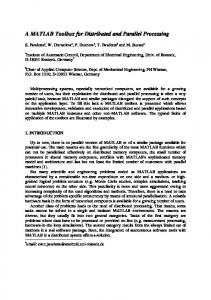
1. Initiate simulations.
2. Simulations transferred to controller.
3. Controller splits simulations into multiple jobs. Client
Controller 4. Jobs are transferred to the agents on the network as they become available.
7. Controller retrieves and collates individual job results and returns them to the client.
6. Agents return job results.
Agents 5. Agents compute a single job with multiple tasks.
Figure 1: Conceptual model of the Apple Xgrid framework (derived from graphic by F. Loxy) which are communicated back to the client by way of R object files created with the R save() function. Much of the work involves specifying a naming structure for the jobs, to allow the results to be automatically collated. The xgrid() function is called to start a series of simulations. This function takes as arguments the R script to run on the grid (by default set to ‘job.R’), the directory containing input files (by default set to ‘input’), the directory to save output created within R on the agent (by default set to ‘output’), and a name for the results file (by default set to ‘RESULTS.rda’). In addition, the number of simulations to run (numsim) and number of tasks per job (ntask) can be specified. The xgrid() function divides the total number of simulations into numsim/ntask individual jobs, where each job is responsible for calculating the specified number of tasks on a single agent (see Figure 1). For example, if 2,000 simulations are desired, these could be divided into 200 jobs each running 10 of the tasks. The number of active jobs on the grid can be controlled using the throttle option (by default, all jobs are submitted then queued until an agent is available). The throttle option helps facilitate sharing a large grid between multiple users. The xgrid() function checks for errors in specification, then begins to repeatedly call the xgridsubmit() function for each job that needs to be created. The xgrid() function also calls The R Journal Vol. X/Y, Month, Year
xgridsubmit() to create a properly formatted ‘xgrid -job submit’ command using Mac OS X through the R system() function. This has the effect of executing a command of the form ‘R CMD BATCH file.R’ on the grid, with appropriate arguments (the number of repetitions to run, parameters to pass along and the name of the unique filename to save results). The results of the system() call are saved to be able to determine the job number for that subtask. This job number can be used to check the status of the job as well as retrieve its results and delete it from the system once it has completed. Once all of the jobs have been submitted, xgrid() then periodically polls the list of active jobs until they are completed. This function makes a call to xgridattr() and determines the value of the jobStatus attribute. The function waits (sleeps) between each poll, to lessen load on the grid. When a job has completed, its results are retrieved using xgridresults() then deleted from the system using xgriddelete(). This capability relies on the properties of the Apple Xgrid, which can be set up to have all files created by the agent when running a given job copied to the ‘output’ directory on the client computer. When all jobs have completed, the individual result files are combined into a single data frame in the current directory. The ‘output’ directory has a complete listing of the individual results as well as the R output from the remote agents. This ISSN 2073-4859
C ONTRIBUTED A RTICLE
ACTION submit attributes results delete
3
R FUNCTION xgridsubmit() xgridattr() xgridresults() xgriddelete()
DESCRIPTION submit a job to the grid controller check on the status of a job retrieve the results from a completed job delete the job
Table 1: Job actions supported by the xgrid command, and their analogous functions in the xgrid package can be useful for debugging in case of problems. To help demonstrate how to access an existing grid, we provide two detailed examples: one involving a relatively straightforward computation assessing the robustness of the one-sample t-test and the second requiring use of add-on packages to undertake simulations of a latent class model. These examples are provided as vignettes within the package. In addition, the example files are available for download from http://www.math.smith.edu/xgrid.
Examples Example 1: Assessing the robustness of the one-sample t-test The t-test is remarkedly robust to violations of its underlying assumptions (Sawiloswky and Blair, 1992). However, as Hesterberg (2008) argues, not only is it possible for the total non-coverage to exceed α, the asymmetry of the test statistic causes one tail to account for more than its share of the overall α level. Hesterberg found that sample sizes in the thousands were needed to get symmetric tails. In this example, we demonstrate how to utilize an Apple Xgrid cluster to investigate the robustness of the one-sample t-test, by looking at how the α level is split between the two tails. This particular study runs very quickly as a loop in R, even for a large number of simulations, and as a result the use of the Xgrid actually slows down the calculation. However, for pedagogical reasons we provide it as a simple example to help describe the setup and test that the Xgrid is functioning appropriately. Our first step is to set up an appropriate directory structure for our simulation (see Figure 5; Appendix A provides an overview of requirements). The first item is the folder ‘input’, which contains two files that will be run on the remote agents. The first of these files, ‘job.R’ (Figure 2), defines the code to run a particular task, ntask times. For this example, the job() function begins by generating a sample of param exponential random variables with mean 1. A one-sample t-test is conducted on this sample, and logical (TRUE/FALSE) values denoting whether the test rejected in that tail are saved in the vectors leftreject and rightreject. This process is repeated ntask times, after which the function job() returns a data frame with the rejection The R Journal Vol. X/Y, Month, Year
results and the corresponding sample size. # Assess the robustness of the one-sample # t-test when underlying data are exponential # this function returns a dataframe with # number of rows equal to the value of "ntask" # the option "param" specifies the sample size job = function(ntask, param) { alpha=0.05 # how often to reject under null leftreject = logical(ntask) # placeholder rightreject = logical(ntask) # for results for (i in 1:ntask) { dat = rexp(param) # generate skewed data left = t.test(dat, mu=1, alternative="less") leftreject[i] = left$p.value