Using a Resource Logic for Multi-Agent Plan Merging - CiteSeerX

Using a Resource Logic for Multi-Agent Plan Merging Mathijs de Weerdt∗, Andr´e Bos†, Hans Tonino, and Cees Witteveen February 27, 2003

Abstract In a multi-agent system, agents are carrying out certain tasks by executing plans. Consequently, the problem of finding a plan, given a certain goal, has been given a lot of attention in the literature. Instead of concentrating on this problem, the focus of this paper is on cooperation between agents which already have constructed plans for their goals. By cooperating, agents might reduce the number of actions they have to perform in order to fulfill their goals. The key idea is that in carrying out a plan an agent possibly produces side products that can be used as resources by other agents. As a result, an other agent can discard some of its planned actions. This process of exchanging products, called plan merging, results in distributed plans in which agents become dependent on each other, but are able to attain their goals more efficiently. In order to model this kind of cooperation, a new formalism is developed in which side products are modeled explicitly. The formalism is a resource logic based on the notions of resource, skill, goal, and service. Starting with some resources, an agent can perform a number of skills in order to produce other resources which suffice to achieve some given goals. Here, a skill is an elementary production process taking as inputs resources satisfying certain constraints. A service is a serial or parallel composition of skills acting as a program. An operational semantics is developed for these services as programs. Using this formalism, an algorithm for plan merging is developed, which is anytime and runs in polynomial time. Furthermore, a variant of this algorithm is proposed that handles the exchange of resources in a more flexible way. The ideas in the paper will be illustrated by an example from public transportation. This report has been published in the Annals of Mathematics and Artificial Intelligence [6].

1

Introduction

1.1

Plan-based controlled agents

One of the design goals of an agent system is to make the programming of the system easier than in conventional systems. Instead of supplying the system with a list of low-level (machine) instructions, an agent is normally told what to do in terms of a high-level goal it has to fulfill. In this way, the user is relieved from the task to program the agent; the agent itself has to find out a way to satisfy the mission goal. Generally speaking, there are two design principles to achieve this kind of behavior: One way is by designing a so-called reactive agent. A reactive agent has a set of rules that given a certain state of the world and the goal to achieve immediately tell the agent what kind of action to perform. In general, the action will change the current state of the world into a new one in which either the goal is satisfied or in which goal satisfaction is easier than in the original situation. Another way to realize goal-finding behavior is to design so-called deliberative agents. Instead of immediately reacting to a new situation, a deliberative agent first tries to find a sequence of actions, or a plan, ∗ Supported

by the Seamless Multimodal Mobility (SMM) research program. by the Freight Transport Automation and Multimodality (FTAM) research program. Both programs are carried out within the TRAIL research school for Transport, Infrastructure and Logistics. † Supported

1

of which the agent can show that it will transform the current situation into one in which the mission goal is satisfied. To facilitate this planning process, each of the agents is equipped with a set of skills or actions that allow them to change the state of the world. Each of these skills can only be applied if the world satisfies a certain condition, that is encoded by a set of required resources of a skill that must be present in the world before a skill may fire. Application of a skill results in producing new resources that may cause other skills to become firable. In this way, a sequence of skills can be constructed such that from an initial situation a desired state of the world can be obtained. In general, the computational burden of a reactive agent is less than that of a deliberative agent, as the solution strategy to satisfy a goal has been designed into the reactive rule set, where a deliberative agent has to compute this strategy for each new situation. The advantage of a deliberative architecture, on the other hand, is that such an agent is able to satisfy a goal also in situations not anticipated during the design of the agent, and that an explicit plan representation can be used for further processing. An explicit plan representation may guide (i) replanning in case contingencies arise during the execution of the plan, and (ii) negotiation if two or more agents want to cooperate, as we describe in this paper.

1.2

Multi-agent systems

Another design goal of an agent system is that it is able to cooperate with other agents. Usually, this requirement stems from the observation that a mission goal cannot be satisfied by a single agent, but requires a joint effort of several agents, coordinating their plans and sharing their resources and goals. Although this observation points out a necessary reason to cooperate, another, almost equally important reason should not be overlooked: Even if agents are able to solve problems on their own, they might prefer to cooperate as sharing their resources and coordinating their activities may save costs or allows them to accept new orders to be executed in parallel. This observation refers to applications such as supply chain management and travel assistance in which individual planning and cooperation phases can be clearly distinguished. For example, a (chain) manager first assigns each agent to a part of a complex task via a task allocation process (see for example the work by Shehory and Kraus [25]), or each agent personally receives some requests by its customers. So, each of the agents has been assigned (sub)goals for which they construct a plan. Finally, the chain manager, or the agents themselves analyze their plans and may try to cooperate in order to satisfy (additional) constraints on costs or performance. In such a case, cooperation can be accomplished by plan revision: to reduce the total cost of his plan an agent tries to revise part of his plan by exchanging resources and goals with other agents.

1.3

Plan merging

Several potential problems may arise during merging of two plans. Plans may conflict because they require the same resource for correct execution, or the prescribed order of actions may lead to dead-lock, e.g., both have to wait for the other to finish a certain action. In order to realistically model real-life situations, we must track different attributes of resources —such as fuel, time, space, and capacity— in a numerical fashion. Furthermore, as one agent may take over responsibility of another one to satisfy a (sub)goal, there must be some form of cost and profit model. In the literature, some attention already has been given to the development and analysis of efficient (approximately or optimal) plan merging methods as discussed in Section 4. We did not encounter, however, computationally feasible approaches for solving the plan merging problem, dealing with the abovementioned, often numerical, constraints.

1.4

Our approach

In this paper, we take a special approach to multi-agent cooperative planning. As in the previously described situation of supply chain management, we assume that each of the agents has a plan

2

available to satisfy their (sub)goals. In order to lower their costs, two or more agents investigate whether they can cooperate. Two agents can cooperate if one agent produces a resource —one that is not directly needed for goal satisfaction, but as a byproduct— that is needed by the other agent. Both agents may agree to cooperate by exchanging resources. That is to say, the agent producing the resource allows the other agent to use it. As a result, the resource that was originally produced as a byproduct becomes a subgoal for the agent. This idea has already been introduced [5, 22], but now we present a thorough logic framework and we show how this process of exchanging resources can be controlled by an auction. We assume one of the agents acts as an auctioneer and collects all requests of all agents. For each request an auction is held, in which all agents, other than the requesting agent, may offer to deliver the requested resource(s). The auctioneer ensures that all constraints are satisfied and that the exchange actually takes place, resulting in a cost reduction. Note that we assume that agents are always willing to cooperate. The structure of this paper is as follows: First, we will introduce a new framework for representing plans. The main features of this framework are (i) the ability to treat plans as first-class citizens, (ii) the distinction between resources, goals and side-products of resource production processes, and (iii) the possibility to model attributes of resources and constraints over attributes in a numerical fashion. We give an operational semantics in terms of a transition system for plans expressed in our resource-based plan formalism. In this framework, we also show that a set of cooperating agents can optimize their plans if they exchange resources. This optimization process is called plan merging. Next, we further investigate this plan merging process by presenting an algorithm for it. We give two variants for the plan merging algorithm: One running in polynomial time, but in which only resources can be exchanged that have similar attributes; and one that is more liberate in that the attribute values need not necessarily be similar, but for which a polynomial running time can not be guaranteed. Finally, we end with a comparison with related work, a description of future work, and conclusions.

2

The resource-skill framework

The formal framework we introduce is built upon three primitive notions: (i) resources, which are the objects manipulated by an agent, (ii) elementary production processes, called skills, used by an agent to consume resources and to produce other resources, and (iii) the goals an agent has to realize. On top of these notions, we introduce resource schemes to represent collections of resources, and services as sequential and independent compositions of skills to model more complex (generic) production processes. We consider services to be the resource production programs an agent might use in order to achieve some goals, given some set of initial resources. Moreover, an agent has the possibility to modify these programs if he is cooperating with other agents to reduce the costs of his service or the costs of the services of other agents. The key ideas we present in this section are the following: 1. We introduce services, which are compositions of skills, as programs an agent can use to realize its goals, given some set of initial resources. A transition system is specified to formalize the operational semantics of these services as programs. 2. It is assumed that skills cannot be used for free. Therefore, an agent will try to reduce the costs of his service by removing one or more skills, while maintaining goal realizability by executing a service reduction process. We present some reduction techniques that maintain goal realizability and hardly affect the structure of the remaining part of the service. As an outcome, we show how goal realizability can be maintained at the cost of increasing serial dependencies between skills. 3. From an abstract point of view, the services of several agents together can be viewed as one aggregated service consisting of the independent composition of the individual agent services. 3

Initially, each of the agents uses its own service to achieve its own goals, independently from the other agents. An agent now has the opportunity to reduce its production costs by removing skills, while maintaining goal realizability, and using some free resources of other agents. As a result, such an agent will become dependent on other agents. In our framework, this means that as a result of such reductions, the original independent composition of services will go through a number of sequential refinements of the aggregated service. We then show that the intra-agent service reduction methods already presented also can be used to model inter-agent cooperation by resource-sharing. 4. Two distinct forms of inter-agent resource sharing are proposed. In the first one, instead of using a service as a generic production process, the specialization (instantiation) of the service w.r.t. the resources and goals given is used. Such “frozen” forms of services are called ground plans. They allow for a restricted, but computationally attractive, form of resource sharing between agents. In the second form, resource sharing is more flexible: instead of using only resources that fit into the current plan, other resources might be used as well, provided that they can be used to realize the current goals of the agent. The results on service and plan reduction will be used in the next section to develop plan and service merging algorithms for agent cooperation. While in the formal framework, we do not distinguish between intra-agent dependencies i.e., dependencies between skills in the service of a single agent, and inter-agent dependencies that relate services of different agents, in these algorithms we will make this distinction. To discuss our framework into detail, first we introduce a many-sorted (resource) language to describe primitive notions like resources, resource schemes, goals and goal schemes. Then we describe skills, services and operations on services. Much of our concepts and notational conventions have been taken from logic programming and are easy to grasp.

2.1

Language

We use a many-sorted first-order language L containing: • Sorts: Sorts = {s1 , s2 , . . . , sn , . . .}; • Variables: Var s = {x1s , . . . , xns , . . .} for each s ∈ Sorts; we use V ar = denote the set of all variables.

S

s∈Sorts

Var s to

• Predicate symbols: P red = {p, q, . . .} with rank r : P red → Sorts ∗ ; • Function symbols: F uns = {f, g, . . .} and rank r : F uns → Sorts + × {s} for each s ∈ Sorts; • Constants: Cons = {c1s , . . . cns , . . .} for each s ∈ Sorts. S Equality is dealt with as usual; the sets Term = s∈Sorts Terms of many-sorted terms and Form of formulae are defined in the usual inductive way, where we distinguish ground terms and ground formulae from general terms and formulae that may contain variables. If x is a variable of sort s, we use x : s to indicate its sort.

2.2

Resources and resource schemes

A resource fact, or simply resource, in our language L, is an L-atomic ground formula p(t1 : s1 , t2 : s2 , . . . , tn : sn ). The terms sj are also called the attributes of resource p with attribute values tj . As an example, take a resource fact taxi(1234 : id, adam : loc, [90, 100] : time) referring to the taxi with identification 1234 at location Amsterdam at time interval [90, 100].1 1 In

this paper we use adam to denote the city Amsterdam and rdam to denote the city Rotterdam.

4

Often, we don’t need to point out a specific individual resource: it is sufficient if the resource we want has certain properties that might be satisfied by more than one specific resource. That is, we are looking for an arbitrary resource belonging to some class of resource facts instead of a specific unique resource. Using the language L, such a class of resources or resource scheme is denoted by a (not necessarily ground) L-atomic formula. Resource schemes are useful to denote arbitrary resources that are ground instances of a resource scheme. For example, taxi(x : id, adam : loc, I : time) is a resource scheme denoting some taxi at Amsterdam, where we don’t care about the time interval I it is available. Given some resource r and a resource scheme rs we would like to know whether r indeed is a ground instance of rs. Hence, we need substitutions. As usual, a substitution θ is a finite set of substitution pairs of the form xi = ti , with xi ∈ Var and ti ∈ Term, satisfying the standard conditions. That is: (i) variables and terms match, i.e., if xi ∈ Vars , then ti ∈ Term s ; (ii) i 6= j implies xi 6≡ xj ; (iii) xi does not occur as a variable in ti . The domain dom(θ) of a substitution θ is the set of variables x for which there exists a substitution pair x = t in θ. If θ and σ are substitutions, θ − σ denotes the set of substitution pairs x = t from θ such that x 6∈ dom(σ). If dom(θ) ∩ dom(σ) = ∅, θ ∪ σ is the substitution consisting of all substitution pairs from θ and σ. A substitution θ is said to be ground, if for every pair of the form xi = ti contained in θ, ti does not contain any occurrence of a variable in V ar. The empty substitution is denoted by . We say that a resource r is an instance of the resource scheme rs if there exists a ground substitution θ such that rsθ = r. If we have a set RS of resource schemes, we would also like to know whether a given set R of resources satisfies RS , i.e., whether R is a typical set of resources denoted by RS . Here we have to be careful: it is not enough to have a substitution θ such that RS θ = R since for each rs ∈ RS we have to find a unique resource r ∈ R as an instance of rs. So an individual resource cannot be used to satisfy more than one resource scheme. Therefore, we do not allow a substitution θ such that for two different schemes rs, rs 0 ∈ RS we have rsθ = rs 0 θ. Hence, we need to introduce resource-identity preserving substitutions: Definition 1 Let RS be a set of resource schemes. A substitution θ is said to be resource-identity preserving w.r.t. RS , if for every rs1 , rs2 ∈ RS , rs1 6= rs2 implies rs1 θ 6= rs2 θ. Hence, an identity-preserving ground substitution w.r.t. RS gives rise to an injection RS → R. It is very easy to check, given a set of resource schemes RS and a substitution θ, whether θ is identity-preserving: Note that for every substitution θ we have |RS θ| ≤ |RS |. By Definition 1, we have |RS θ| ≥ |RS |. Hence, if θ is resource-identity preserving, then |RS | = |RS θ|. Analogously, if θ is a substitution such that |RS | = |RS θ|, it immediately follows that rs1 6= rs2 implies rs1 θ 6= rs2 θ. Summarizing this line of reasoning, we have: Proposition 1 A substitution θ is resource-identity preserving w.r.t. a given set of resource schemes RS iff |RS | = |RS θ|. Definition 2 A set of resources R satisfies a set RS of resource schemes, denoted by R |= RS , if there exists a resource-identity preserving ground substitution θ w.r.t. RS , such that RS θ ⊆ R. To indicate the substitution θ explicitly, we write R |=θ RS . Sometimes, we need to find a collection of resources that not individually, but together satisfy some conditions. Corresponding classes of resources can be obtained by introducing extended resource schemes: Definition 3 An extended resource scheme is a tuple (RS , C), where (i) RS is a set of resource schemes, and (ii) C is a set of constraints for terms with variables occurring in resources in RS . 2 2 We

do not feel the need to specify exactly the type of constraints we will use; it suffices to use standard relations.

5

Remark 1 Note that every set R of resources is a special set of resource schemes. An arbitrary set RS of resource schemes is a special case of an extended resource scheme, where the set C of constraints equals {true}. Of course, we would also like to know whether a given set R of resources satisfies a set of extended resource schemes RS : Definition 4 A set of resources R satisfies an extended resource scheme (RS, C), abbreviated as R |= (RS, C), if there exists some resource-identity preserving ground substitution θ w.r.t. RS such that 1. RSθ ⊆ R, 2. |= Cθ, i.e., every constraint reduces to true under θ. If we want to specify the substitution θ used to satisfy the extended resource scheme, we write R |=θ (RS, C). To give an example, consider a passenger p(x1 : loc, I1 : time) at location x1 at time interval I1 , waiting for a (taxi)-ride ride(x2 : loc, y : loc, c : cap, I2 : time) from location x2 to y, having c free seats and occurring in time interval I2 . To help the passenger it is required that x1 = x2 , c > 0, and I1 ∩ I2 6= ∅. This is expressed by the following extended resource scheme: ( {p(x1 : loc, I1 : time), ride(x2 : loc, y : loc, c : cap, I2 : time)}, {x1 = x2 , I1 ∩ I2 6= ∅, c > 0} ) Every set R of resources containing at least one ride and one passenger resource meeting these constraints will satisfy this extended resource scheme. In this example we used x1 and x2 to denote the same location, because of the constraint x1 = x2 . Later in this paper we will use only one variable x and omit this constraint.

2.3

Goals

Some resources an agent already has, others he needs to obtain. In general, such an agent does not care about obtaining a specific (unique) resource as a goal g, but only a resource having some specific properties. So we will conceive an individual goal g as a resource scheme. Even more generally, we may want to obtain a set of goals meeting some constraints. Therefore, we define goals and goal schemes analogously to resources and extended resource schemes as follows: Definition 5 A goal g is a resource scheme. A goal scheme Gs is an extended resource scheme Gs = (G, C), where G is a set of goals. As goal schemes are extended resource schemes, we also use R |= Gs to express that the resource set R satisfies the goal scheme Gs.

2.4

Skills

Suppose we are given some set of resources R and we want to obtain some set of resources R0 satisfying a given goal scheme Gs. We clearly need a way to transform the set R into this set R0 . To this end, we introduce skills as (elementary) resource consuming and resource production processes: Definition 6 A skill is a rule of the form s : RS 0 ← (RS , C). Here, s is the name of the skill, RS 0 is a set of resource schemes containing only variables that occur in the extended resource scheme (RS , C), i.e., var(RS 0 ) ⊆ var(RS).

6

Intuitively, the meaning of a skill s is as follows: whenever there is a set of resources R and a ground substitution θ such that R |=θ (RS , C), the set R is consumed by s and a new set of resources R0 = RS 0 θ will be produced.3 This set R0 is uniquely determined by θ and RS. We identify the set of constraints C occurring in a skill s by Cs . Furthermore, var(s) = var(RS) denotes the set of variables occurring in s, in(s) = RS denotes the set of input resource schemes, and out(s) = RS 0 is the set of output resource schemes. Definition 7 Skill application to resources: Let s : RS 0 ← (RS , C) be a skill and let R, R0 be sets of resources. We say that R0 can be produced from R using s, abbreviated by R `s R0 , if there is a resource-identity preserving ground substitution θ w.r.t. RS ∪ RS 0 such that4 1. R |=θ RS , 2. |=θ C, i.e., every constraint in C reduces to true under θ, and 3. R0 = (R − RS θ) ∪ RS 0 θ, i.e., the resources RS θ which are consumed by s are removed from R, while the resources RS 0 θ produced by s are added to the remaining set of resources. Example 1 To give two concrete examples, take the following skills: drive rdam : taxi(rdam : loc, [t1 + t(x, rdam), t2 ] : time), ride(x : loc, rdam : loc, 2 : cap, [t1 , t2 ] : time) ← (taxi(x : loc, [t1 , t2 ] : time), ∅) travel :

p(y : loc, [t3 + t(x, y), t2 ] : time) ← (p(x : loc, [t1 , t2 ] : time), ride(x : loc, y : loc, c : cap, [t3 , t3 ] : time), {t1 ≤ t3 , t3 + t(x, y) ≤ t2 , c ≥ 1})

To explain the last skill, travel: for a passenger to travel from location x to location y, two resources are needed. First of all, the passenger should be at location x at a certain time t1 and secondly, a ride (produced by a taxi) should be available at a time t3 ≥ t1 and with capacity at least 1. The time the passenger arrives at location y is calculated using a pre-defined time-distance matrix t(x, y). The constraint t3 + t(x, y) =< t2 ensures that the passenger arrives before his deadline t2. A ride resource can be produced by the first skill: Take the resource set R = {taxi(adam, [10, ∞])}, suppose that t(adam, rdam) = 40 and let θ = {x = adam, t1 = 10, t2 = ∞}. Then {taxi(adam, [10, ∞])} `drive rdam {taxi(rdam, [50, ∞]), ride(adam, rdam, 2, [10, 10])}. Skills represent generic production processes that may be applied to different sets of resources. Since the same skill may be used more than once, we should be able to distinguish several uses of the same skill; therefore we introduce skill variants: Definition 8 Two skills s1 : RS 01 ← (RS 1 , C1 ) and s2 : RS 02 ← (RS 2 , C2 ) are said to be variants if there exist substitutions θ and ψ such that 1. RS 01 θ = RS 02 , RS 1 θ = RS 2 , C1 θ = C2 , 2. RS 02 ψ = RS 01 , RS 2 ψ = RS 1 , C2 ψ = C1 , and 3. var(s1 ) ∩ var(s2 ) = ∅. It is not difficult to see that whenever two skills s1 and s2 are variants, the substitutions θ and ψ involved have to be resource-identity preserving w.r.t. RS 1 ∪ RS 01 and RS 2 ∪ RS 02 , respectively.5 3 That is, every skill is range restricted, meaning that from ground resources only ground resources can be produced. 4 Note that by Proposition 1 this immediately implies that θ is identity-preserving w.r.t. RS as well as w.r.t. RS 0 . 5 It suffices to observe that RS 0 θ = RS 0 implies |RS 0 | ≥ |RS 0 | and RS 0 ψ = RS 0 implies |RS 0 | ≥ |RS 0 |. Hence, 1 2 1 2 2 1 2 1 |RS 01 | = |RS 02 | = |RS 01 θ|, implying that θ is resource-identity preserving w.r.t. RS 01 . Analogously for RS 1 , RS 02 and RS 2 .

7

2.5

Resources, skills and uniqueness postulates

As remarked before, resources are considered to be unique objects in our framework. Since we are dealing with skills that consume and produce resources, it is not sufficient to deal with uniqueness in a (current) set of resources. Instead, we want uniqueness to be preserved also in these generic resource consumption and production processes. We capture these uniqueness requirements in the form of the following uniqueness postulates: Postulate UN1. Every resource r is a unique object, uniquely identified by a resource fact. Postulate UN2. Whenever a resource r has been consumed by a skill application it can never be reproduced by any sequence of skill applications. Postulate UN3. A resource r produced by a a skill variant s is uniquely determined by s and the unique input resources of s. Postulate UN4. A skill is a generic production process. A goal is a generic resource object. Therefore, a skill can never require a unique resource to be given as one of its input resources and a goal can always be satisfied by more than one possible resource. These uniqueness postulates can be satisfied if every resource has a special identification attribute id. For each resource r, the id attribute has a unique value. We also consider a countable set of skill(variants); each such a skill variant has a unique identification number. Whenever a resource r appears as output of a skill, the value of the id attribute of r is determined by the concatenation of the values of the input identification labels and the skill-identification number. Hence, the value of the identification attribute of a resource r will reflect its production history and — given unique initial values of input resources — we are guaranteed to preserve uniqueness of every resource ever produced or consumed. Note that the last postulate requires that we can never use specific values of the id-attribute as one of the constraints on the variables of input resources. In fact, it is sufficient to assume that the id attribute is never mentioned in the set of constraints of a skill s or goal scheme. In the sequel, we assume that every resource has such an identification attribute id and we define two resources to be similar if they are identical with the possible exception for the value of their id-attributes. Definition 9 Resources r, r0 having the same predicate name and attributes and attribute values, with the possible exception of values of the id attribute, are said to be similar resources, abbreviated as r ≈ r0 . Analogously, if there exist resource sets R, R0 and a bijection f : R → R0 such that for every r ∈ R, r ≈ f (r), we say that R is similar to R0 , abbreviated as R ≈ R0 . Analogously, for substitutions σ and σ 0 , we write σ ≈ σ 0 if they are identical with the possible exception of the values assigned to the id-attribute. Note that according to Postulate UN3, similar resources are indistinguishable for skills or goals.

2.6

Services

In general, most of the goals are not realizable by applying just a single skill on the set of available resources. Instead they will require the execution of several skills sequentially and/or concurrently to reach some goals. OfScourse, we might use Definition 7 and the transitive closure of the production relation `S = s∈S `s to describe the set of resources sets R0 derivable from a given resource set R. However, we will not do so. The reason is that we are not primarily interested in finding the skills to produce a set of resources from an initial set of resources —this surely is a difficult planning problem—, but in using a given (structured) set of skills to produce a set of resources.

8

Instead of determining a complete plan from scratch, we assume the existence of such a skill program, also called a service, and we will use these services to test whether they can be used to obtain some given goal, and, if so, whether they can be simplified to reach these goals. We will assume that such a service consists of a composition of (unique) skills or variants of skills. The set of services Ss over the set S of skill(variant)s is inductively defined as follows: Definition 10

1. E is a service over ∅, called the empty service;

2. every skill s is a service over the set {s}; 3. if π1 and π2 are services over S1 and S2 and S1 ∩ S2 = ∅, then (π1 ; π2 ) and (π1 k π2 ) are services over S1 ∪ S2 . Here ; denotes sequential composition and k denotes the independent composition operator. The service π1 ; π2 expresses that starting the execution of skills in π2 is dependent upon completion of all skills in π1 , while π1 k π2 denotes two services that have to be executed completely independent from each other, that is, no resource produced or consumed by π1 can be consumed by a skill in π2 and vice-versa and there are no execution constraints between skills in the two services. If Ss is a service over a set S of skills, Skills(Ss) = S denotes the set of skills used in Ss. Without loss of generality, we can always assume that whenever s, s0 ∈ Skill(Ss) are two different skills then var(s) ∩ var(s0 ) = ∅.

2.7

A transition system specification for services

A service Ss is a kind of program an agent can execute on a given set R of resources to obtain some set of goals. During execution of skills in a service, the agent creates new sets of resources that in turn might be changed by executing the remaining part of the service. So we identify a state of an agent A by a tuple (Ss, R) where Ss is the (remaining part of a) service to be applied on the current set of resources R. After successful execution of the complete service Ss, its final state will be (E, R0 ) for some set of final resources R0 . To specify a transition relation between the states of an agent and especially between initial states (Ss, R) and final states (E, R0 ), we use transition systems (cf. [23]) to define the operational semantics of skill applications, sequential composition and independent composition. Each of the following definitions specifies a transition rule defining the results a single skill application, and the composition operators have on the current state of the agent. Together they inductively define the transition relation → between the states of an agent. During the execution of skills, the agent creates substitutions θ used to bind skill variables to attribute values in resources. For bookkeeping purposes, we will often use such substitutions as subscripts in the transition relation →. First of all, we need reflexivity: by using an empty substitution, a transition can be made from a state to itself. Definition 11 Reflexivity (π, R) → (π, R) Given a skill s and a set of resources R, the skill can be executed on R whenever we can find an identity preserving ground substitution θ that (i) satisfies the constraints Cs and (ii) applied to in(s) selects a subset of the resources (cf. Definition 7): Definition 12 Transition rule for skill application in(s)θ ⊆ R, |=θ Cs , R0 = (R − in(s)θ) ∪ out(s)θ (s, R) →θ (E, R0 )

9

The sequential composition π1 ; π2 of two services π1 and π2 using resources in R requires the execution of all skills in π1 on R (resulting in an intermediate set of resources produced), before π2 can be applied. We distinguish two cases: One to execute (part of) π1 (Definition 13) and one to execute π1 and (a part of) π2 (Definition 14). Definition 13 Transition rule for sequential composition — reduction (π1 , R) →θ (π10 , R0 ) →θ0 (E, R00 ) (π1 ; π2 , R) →θ (π10 ; π2 , R0 ) Definition 14 Transition rule for sequential composition — elimination (π1 , R) →θ1 (E, R00 ) , (π2 , R00 ) →θ2 (π20 , R0 ) →θ20 (E, R000 ) (π1 ; π2 , R) →θ1 ∪θ2 (π20 , R0 ) Note that these two rules define any state transition for a sequential composition of services, so we do not need the transitive closure of →. The specification of the independent composition π1 k π2 using resources in R is somewhat more involved. The reason is that this operator is used to express that two sub-services (i) have to be completely independent w.r.t. their resource needs and (ii) run concurrently. These concurrency aspects, however, have to be specified by the independent and successful execution of the subservices separately. Definition 15 Transition rule for independent composition — reduction (π1 , R1 ) →θ1 (π10 , R10 ) →θ10 (E, R100 ), (π2 , R2 ) →θ2 (π20 , R20 ) →θ20 (E, R200 ), R1 ∩ R2 = ∅ (π1 k π2 , R1 ∪ R2 ) →θ1 ∪θ2 (π10 k π20 , R10 ∪ R20 ) We note that if R1 ∩R2 = ∅, as a consequence of the uniqueness postulates, we also have R10 ∩R20 = ∅. Finally, we need two transition rules to deal with the borderline cases E k π and π k E to identify them with π: Definition 16 Transition rules for E k π and π k E — elimination (π, R) →θ (π 0 , R0 ) (π, R) →θ (π 0 , R0 ) , (E k π, R) →θ (π 0 , R0 ) (π k E, R) →θ (π 0 , R0 ) Example 2 Consider the drive and travel skills discussed before. Let Ss be the set {drive rdam, travel} and let R be the following set of resources {taxi(adam, [100, ∞]), p(adam, [80, ∞])}. Using the transition specifications defined in Definition 12 we derive: (drive rdam, {taxi(adam, [100, ∞]), p(adam, [80, ∞])}) →θ1 (E, {taxi(rdam, [140, ∞]), ride(adam, rdam, 2, [100, 100]), p(adam, [80, ∞])}) and (travel, {taxi(rdam, [140, ∞]), ride(adam, rdam, 2, [100, 100]), p(adam, [80, ∞])}) →θ2 (E, {taxi(rdam, [140, ∞]), ride(adam, rdam, 1, [100, 100]), p(rdam, [140, ∞])}) and thus by Definition 14 and reflexivity: (Ss, R) →θ1 ∪θ2 (E, {taxi(rdam, [140, ∞]), ride(adam, rdam, 1, [100, 100]), p(rdam, [140, ∞])}) where θ1 = {x = adam, t1 = 100, t2 = ∞} and θ2 = {x = adam, y = rdam, t1 = 80, t2 = ∞, t3 = 100, c = 2}. 10

Using the transition rules defined, we now use → as the reflexive closure of the relation specified by these rules. As an immediate consequence of the preceding definitions and the uniqueness postulates, we mention the following properties of the relation →: Proposition 2 If (π, R) →θ (π 0 , R0 ) then 1. (resource monotony) for every set of resources R1 , (π, R ∪ R1 ) →θ (π 0 , R0 ∪ R1 ); 2. (irrelevance of unused resources) (π, R − R00 ) →θ (π 0 , R0 − R00 ) for every R00 ⊂ R ∩ R0 ; 3. (resource production genericity) if R1 ≈ R then there exists some R10 ≈ R0 and a substitution θ0 ≈ θ such that (π, R1 ) →θ0 (π 0 , R10 ). Proof 1 By easy induction on the structure of the service π.

2.8

Goal satisfaction, service reduction and sequential refinement

Given these transition rules, we now are able to define whether a goal scheme Gs can be satisfied by a service Ss: Definition 17 Let Ss be a service over the set S, R a set of resources and Gs = (G, C) a goal scheme. We say that (Ss, R) satisfies Gs, abbreviated as (Ss, R) |= Gs, if there exists an R0 such that (Ss, R) → (E, R0 ) and R0 |= Gs. If (Ss, R) →θ (E, R0 ), R0 |=σ Gs and we want to specify these substitutions explicitly, we write (Ss, R) |=θ,σ Gs. 2.8.1

Service reduction

Using a service Ss to obtain some goals, it may be the case that not every skill occurring in Ss is needed to satisfy the goals. If the use of a skill is not for free, it might be profitable for an agent to look for skills that might be omitted from a service if the goals and initial resources are known. In this subsection we will develop some results about such service reduction methods. In particular, we will study the consequences of removing one skill from a service, while leaving nearly untouched the remaining structure of the service. Definition 18 Let Ss be a service and s a skill occurring in Ss. The elementary reduction of Ss w.r.t. s, denoted by Ss − s, is the service obtained from Ss by substituting E for s in Ss. Given a service Ss and a set S = {s1 , . . . , sn } of skills, the reduced service Ss − S is obtained by repeatedly removing a skill from S from Ss. First we show that the loss of a skill in a service can be easily compensated by adding the right resources in order to maintain goal realizability. Intuitively, these additional resources should be similar to the output resources of the skill. We will use this result further on and therefore we present a rather elaborate proof. Proposition 3 If (Ss, R) |=θ,σ Gs and s is a skill occurring in Ss, then (Ss−s, R∪out(s)τ ) |=(θ−τ ),σ Gs, where τ ⊂ θ is a substitution with dom(τ ) = var(s). Proof 2 By induction on the structure of Ss we show that (Ss, R) →θ (E, R0 ) for some substitution θ, implies that there exists some substitution τ ⊂ θ with dom(τ ) = var(s), such that (Ss − s, R ∪ out(s)τ ) →θ−τ (E, R0 ∪ in(s)τ ). Then (Ss, R) |=θ,σ Gs implies that R0 ∪ in(s)τ |=σ Gs and therefore, (Ss − s, R ∪ out(s)τ ) |=(θ−τ ),σ Gs. So it remains to present the proof by induction. 11

1. Suppose Ss = s and (s, R) →θ (E, R0 ) for some substitution θ. By Definition 12, it follows that R0 = (R − in(s)θ) ∪ out(s)θ. Since → is reflexive, and τ = θ, (Ss − s, R ∪ out(s)θ) = (E, R ∪ out(s)θ) → (E, R ∪ out(s)θ) = (E, R0 ∪ in(s)θ). 2. Suppose Ss = (π1 ; π2 ) and (Ss, R) →θ (E, R0 ). Hence, we have (π1 ; π2 , R) →θ1 (π2 , R00 ) →θ2 (E, R0 ) where θ = θ1 ∪ θ2 . But this implies that (π1 , R) →θ1 (E, R00 )

(1)

(π2 , R00 ) →θ2 (E, R0 )

(2)

and We distinguish two cases: (a) If s ∈ Skills(π1 ), then, by induction hypothesis, we derive from equation (1): (π1 − s, R ∪ out(s)τ ) →θ1 −τ (E, R00 ∪ in(s)τ ) where τ ⊂ θ1 . By monotonicity (see Proposition 2 (i) ), it follows from Equation (2) that (π2 , R00 ∪ in(s)τ ) →θ2 (E, R0 ∪ in(s)τ ) and combining these derivations, noting that Ss − s = (π1 − s; π2 ), we derive (Ss − s, R ∪ out(s)τ ) →θ−τ (E, R0 ∪ in(s)τ ). (b) If s ∈ Skills(π2 ), then, by induction hypothesis, we have (π2 − s, R00 ∪ out(s)τ ) →θ2 −τ (E, R00 ∪ in(s)τ ) where τ ⊂ θ. But then, again by Proposition 2 (i) and by equations (1) and (2), it follows that (Ss − s, R ∪ out(s)τ ) →θ−τ (E, R0 ∪ in(s)τ ). 3. Suppose Ss = π1 k π2 and (Ss, R) →θ (E, R0 ). By the definition of k we must have R = R1 ∪ R2 for some R1 , R2 and (π1 , R1 ) →θ1 (E, R10 ) and (π2 , R2 ) →θ2 (E, R20 ) where θ = θ1 ∪ θ2 and R0 = R10 ∪ R20 . Without loss of generality we may assume that s ∈ Skills(π1 ). Hence, by induction hypothesis, (π1 − s, R1 ∪ out(s)τ ) →θ1 −τ (E, R10 ∪ in(s)τ ). where τ ⊂ θ1 . By the uniqueness postulates UN1 - UN3, it follows that (R1 ∪out(s)τ ) ∩ R2 = ∅ and (R10 ∪ in(s)τ ) ∩ R20 = ∅. Hence, using Definition 15, we derive (Ss − s, R ∪ out(s)τ ) →θ−τ (E, R0 ∪ in(s)τ ). This proposition captures the intuitively obvious idea that a loss of some skill in a service always can be compensated for by (i ) adding some (initial) resources, (ii ) without affecting the structure of the remaining part of the service. In general, however, this is not a solution we are interested in. Instead, we would like to find a solution (i ) without affecting the initial set of resources available and (ii ) hardly affecting the structure of the remaining part of the service. The idea is that sometimes we do not need to add resources if we can use resources produced by the service Ss itself that are not involved in the goal satisfaction process. That is, whenever 12

we remove a skill s we might try to compensate for its removal by using free resources generated by other skills in the service to substitute for the output resources of s. To guarantee that such a substitution of resources does not affect the goal realizability when executing the remaining part of the service, we have to analyze what requirements such resources have to satisfy in order to be used. This will force us to analyze the dependency structure between a given skill and other skills in a service. Secondly, we have to make clear what is meant by a hardly changing the structure of the remaining service in order to adapt to the loss of some skill. To this end we will introduce the notion of a sequential refinement of a service. 2.8.2

Free resources and dependencies

Suppose some skill s is removed from Ss and let r be a resource produced by s that is used as input resource of some skill s0 sequentially dependent on s. So we need to replace r. Suppose that a resource r0 produced by some skill s00 , is used to replace r. As a consequence, a sequential dependency will be created between s00 and s0 . This immediately implies that the production of such a free resource r0 should not depend on the skill s nor on any skill sequentially dependent on s in the service Ss. So, let Ss be a service containing a skill s. We define the (sub)service Sspost(s) as the service containing all skills in Ss dependent on s, as follows: Definition 19

Sspost(s)

 E    0   (πpost(s) ; π ) 0 πpost(s) =    πpost(s)   0 πpost(s)

if if if if if

Ss = s, Ss = (π; π 0 ) and s occurs in π, Ss = (π; π 0 ) and s occurs in π 0 , Ss = (π k π 0 ) and s occurs in π, Ss = (π k π 0 ) and s occurs in π 0 .

As an easy consequence of the last definition we mention the following proposition: Proposition 4 If s ∈ Skills(Ss) and s0 ∈ Skills(Sspost(s) ) then Skills(Sspost(s 0 ) ) = Skills((Sspost(s) )post(s 0 ) ) ⊆ Skills(Sspost(s) ). It follows that no resource produced by a skill in Sspost(s) can be used as a free resource to compensate for the removal of s from Ss. Now we are ready to define the set of free resources F ree(Ss, s, R, θ) that might be used to replace resources r produced by some skill s removed from Ss: Definition 20 Let (Ss, R) →θ (E, R0 ) and s ∈ Skills(Ss). The set of free resources F ree(Ss, s, R, θ) that can be used if s is removed from Ss equals the set Rf ree satisfying (Ss, R) →θ (s; Sspost(s) , Rf ree ). That is, the set Rf ree equals the set of resources produced by the part of the service Ss not containing s or any service sequentially dependent on s in Ss using the original bindings θ that have been produced when Ss was applied to R. 2.8.3

Sequential refinement

We use a sequential refinement of a service to capture the idea of minimal changes in the structure of a service. Intuitively speaking, Ss 0 is a sequential refinement of Ss iff sequential precedence constraints in Ss are not violated. This notion can be easily defined using the set of dependencies in a service. Definition 21 Let Ss and Ss0 be services. Then Ss 0 is a sequential refinement of Ss, abbreviated Ss0  Ss, iff

13

1. Skills(Ss) = Skills(Ss 0 ), 0 2. for every s ∈ Ss, Skills(Sspost(s) ) ⊆ Skills(Sspost(s) )), 0 i.e., Ss respects all sequential dependencies occurring in Ss.

An important property of sequential refinements is that the transition relations are preserved: Lemma 1 Sequential refinement and transition relation: If it holds that (Ss, R) →θ (E, R0 ) and Ss0  Ss then (Ss0 , R) →θ (E, R0 ). Proof 3 Easy but tedious by induction on the composition of Ss. Using these notions of refinements and free resources, we will state now one of the main results of this section. The following theorem characterizes (i ) the requirements a set of free resources has to satisfy and (ii ) the changes that have to be made in the remaining part of the skill in order to guarantee goal realizability. Intuitively, the theorem states that whenever a skill s is removed from a service Ss used and the set of free resources is sufficient to realize the goal starting with the sub service Sspost(s) , we always can find a sequential refinement of Ss − s that realizes Gs using the original set of resources. Theorem 1 Let (Ss, R) |=θ,σ Gs, s ∈ Skills(Ss) and Fs be the set of free resources F ree(Ss, s, R, θ). If (Ss post(s) , Fs ) |= Gs, there exists a sequential refinement Ss0  (Ss−s) such that (Ss0 , R) |= Gs. Proof 4 Suppose the conditions are verified. So, let (Ss, R) |=θ,σ Gs, s ∈ Skills(Ss), Fs = F ree(Ss, s, R, θ) and suppose (Sspost(s) , Fs ) |= Gs. We define the service Sspre to be the subservice obtained from Ss by substituting E for every skill occurring in {s} ∪ Skills(Sspost(s) ) and we define the service Ss0 as the sequential composition of Sspre and Sspost = Sspost(s) : Ss0 = (Sspre ; Sspost ). It now suffices to verify the following claims: Claim 1. Ss0  (Ss − s); i.e., Ss0 is a sequential refinement of Ss; Claim 2. (Ss0 , R) |= Gs. Ad Claim 1. By definition of Ss0 , it immediately follows that Skills(Ss0 ) = Skills(Ss − s). Let s0 be an arbitrary skill in Ss − s. We verify that Skills((Ss − s)post(s0 ) ) ⊆ Skills(Ss0post(s0 ) ), distinguishing the following cases: • s0 occurs in Sspre . Then Skills((Ss − s)post(s0 ) ⊆ Skills((Sspre )post(s0 ) ) ∪ Skills(Sspost(s) ) = Skills(Ss0post(s0 ) ). • s0 occurs in Sspost . Then we have Skills((Ss − s)post(s0 ) ) = Skills((Sspost )post(s0 ) ) = Skills(Ss0post(s0 ) ). Therefore, Ss0  (Ss − s).

14

Ad Claim 2. Since Fs = F ree(Ss, s, R, θ), by definition, it follows that (Ss, R) →θ (s; Sspost(s) , Fs ). Hence, according to the definition of Sspre we have (Ss − Skills(s; Sspost(s) ), R) = (Sspre , R) →θ1 (E, Fs ). where θ1 ⊂ θ is the restriction of θ to var(Sspre ). Now assuming that (Sspost(s) , Fs ) |= Gs, there exists a substitution σ and a set of resources R0 such that (Sspost(s) , Fs ) →σ (E, R0 ) and R0 |= Gs. Since Ss0 = (Sspre ; Sspost(s) ) we now immediately derive that (Ss0 , R) →θ1 ∪σ (E, R0 ) and therefore, (Ss0 , R) |= Gs. Observe that θ1 ∪ σ does not need to be contained in θ. The reason is that a completely different set of bindings might be produced by Sspost(s) to derive a set of resources satisfying Gs. There is, however, a special case in which the same bindings used in the execution of Ss can be used to satisfy the set of goals in the reduced service. Suppose that a service Ss is used to produce a set of resources R0 from R using a substitution θ. Moreover, it is known that R0 |=σ Gs. Let s be a skill to be removed and let Fs the set of of free resources not depending on s. Suppose now that we are able to find a set of resources Rs similar to the set out(s)θ of resources to be replaced such that (i ) Rs contains output resources of Ss or input resources of s i.e., Rs ⊆ (Fs ∩ R0 ) ∪ in(s)θ and (ii ) Rs is not involved in the binding of goals, that is: R0 − Rs |=σ Gs. We show that we can use Rs to replace the resources originally produced by s if we use a sequential refinement of Ss − s: Theorem 2 Let (Ss, R) →θ (E, R0 ), R0 |=σ Gs, s ∈ Skills(Ss) and let Fs = F ree(Ss, s, R, θ) be the set of free resources. If there is a set Rs ⊆ (Fs ∩ R0 ) ∪ in(s)θ such that 1. Rs ≈ out(s)θ and 2. (R0 − Rs ) |=σ Gs, then there exists a sequential refinement Ss0  Ss − s such that for substitutions θ0 ≈ θ and σ 0 ≈ σ it holds that (Ss0 , R) |=θ0 ,σ0 Gs. Proof 5 Suppose that all the conditions hold. Let Sspre = (Ss − s) − Skills(Sspost(s) ). From the definition of Fs it follows that (Ss, R) →θ1 (Ss − Sspre , Fs ) where θ1 is θ restricted to Sspre . But this implies that (Sspre , R) →θ1 (E, Fs ). Define the service Sss = Ss pre ; s; Ss post(s) . Clearly, Ss is a sequential refinement of Ss and by Lemma 1, we have (Sss , R) →θ1 (s; Sspost(s) , Fs ) →θ−θ1 (E, R0 ) Then it suffices to prove that (Sspost(s) , Fs ) |=ρ,σ0 Gs for some ρ ≈ (θ − θ1 ) and σ 0 ≈ σ. Since (s; Sspost(s) , Fs ) →θ−θ1 (E, R0 ), by Proposition 3 it follows that (Sspost(s) , Fs ∪ out(s)τ ) →θ−θ1 −τ (E, R0 ∪ in(s)τ ) where dom(τ ) = var(σ). Since Rs ⊆ (R0 ∩ Fs ) ∪ in(s)θ, by Proposition 2 (2) we also have (Sspost(s) , Fs ∪ out(s)τ − Rs ) →θ−θ1 −τ (E, R0 ∪ in(s)τ − Rs ) Now out(s)θ ≈ Rs and since τ equals θ restricted to var(s), we also have out(s)τ ≈ Rs . Therefore, by Proposition 2 (3): (Sspost(s) , Fs ∪ Rs − Rs ) →θ−θ1 −τ (E, R00 ) 15

where R00 ≈ (R0 ∪ in(s)θ − Rs ). Hence, (Sspost(s) , Fs ) →θ−θ1 −τ (E, R00 ). Finally, since (R0 − Rs ) |=σ Gs, we also have R0 ∪ in(s)θ − Rs ) |=σ Gs. But then, by postulate UN3, it follows that R00 |=σ0 Gs for some σ ≈ σ 0 . Using ρ = θ − θ1 , we have (Sspost(s) , Fs ) |=ρ,σ0 Gs.

2.9

Sequential refinement and multi-agent cooperation

The elementary reductions of services can be applied to the services of single agents but also —in a more interesting way— to the services of agents together. Suppose that A1 , . . . , An are agents using (disjoint) sets of resources Ri and services Si to satisfy goal schemes Gsi = (Gi , Ci ). Clearly, an independent combination Ss = Ss1 k Ss2 . . . k Ssn of their services can be considered as a model of their joint services and we can easily derive [ [ (Ss, R1 ∪ R2 . . . ∪ Rn ) |= ( Gi , Ci ). S S That is, the agents jointly are able to satisfy the joint goals Gs = ( Gi , Ci ) using their joint resources R = R1 ∪ R2 . . . ∪ Rn . Hence, the service reduction techniques discussed sofar for the single agent case can be easily extended to deal with the multi-agent case and can be used to form the formal basis for modeling agent cooperation, if we are prepared to model both intra- and inter-agent independent skill execution using the independent combination operator k. Imagine that, initially, the agents run their services concurrently to satisfy their individual goals. We assume that the cost of executing a service is the sum of the costs associated with the applications of the individual skills and the costs of the resources occurring in R. Although the concurrent composition of services is sufficient to satisfy the goals, it will often contain more skills and uses more resources than is necessary to satisfy all the goals. Hence, the agents might try to reduce the costs of their service by (i ) reducing the number of skill applications (ii ) without increasing the set of resources available, while (iii ) maintaining goal-realizability. The techniques they can apply essentially are based on the service reduction theorems we have presented above. Basically, we distinguish two main techniques for inter-agent cooperation: 1. Ground-plan based merging. In the previous section we used a service Ss to apply them to a resource set R thereby generating a ground substitution θ and producing a set of resources R0 . This set in turn was shown to satisfy a given goal scheme Gs = (G, C) by using a substitution σ such that Gσ ⊆ R0 while |= Cσ. It is not difficult to see that Ssθ is an independent/sequential composition of ground instances of skills taking as input a set of resources R and producing R0 . The substitution σ informs us in a unique way about the subset Gσ of R0 that is used to satisfy the goal scheme. We call the triple (R, Ssθ, Gσ) a ground plan for achieving Gs from R using θ. Assuming that all the agents have such ground plans for realizing their goals, they might try to reduce their ground plans, that is try to remove some of the ground instances of the skills used, without affecting the substitutions used in other skills and the goal bindings. Such reductions can only be achieved if upon the removal of such a ground instance sθ, the agent can find a set of resources similar to out(s)θ if sθ is used in the goal production. Theorem 2 provides the essentials of such ground-plan based merging processes. 2. Flexible-plan based merging While ground-plan based merging can be achieved rather efficiently, in many respects it is rather inflexible. Sometimes, an agent might use resources of another agent after a removal of its own skill, but then he has to adapt some of the remaining skill applications because the resources provided are not similar to the ones to be replaced. They even might have some consequences in the goal to end-product bindings. Merging techniques based on an exchange of non-similar resource sets can be based on Theorem 1. These merging techniques

16

require the use of the original skill and testing of constraints. It is therefore more flexible, but in general computationally more involved. We will discuss both variants in the next section. Example 3 Consider again the drive and travel skills discussed before, let Ss = {drive rdam; travel} and let t(adam, rdam) = 40. Furthermore, let R = ({taxi(adam, [100, ∞]), p(adam, [80, ∞])} be a set of resources, and (G, C) = ({p(rdam, [t00 , ∞])}, {t00 ≤ 150)}) be a goal scheme. Then P = (R, Ssθ, Gσ) with θ = {x = adam, y = rdam, t1 = 100, t2 = ∞, t3 = 100, c = 2} and σ = {t00 = 140} is a is a ground plan for (G, C) using Ss.

3

Plan merging

For agents acting in a common environment, on one hand, it is often necessary to cooperate, for example, to reduce their costs. On the other hand, agents usually like to keep some information to themselves. The following example illustrates this difficulty. Example 4 Consider two taxi companies each having their own plans for their taxis. Such companies do not like to reveal all their plans to a third party, because they don’t trust each other, but they do like to cooperate, because taxis often drive to a location without transporting any passengers. It may happen that such an empty ride coincides with the route one of the clients of the other company would like to take. In this case, one company could sell its —otherwise unused— ride to the other, thereby reducing the costs of its plan. In the previous section, we have shown that a skill can be deleted from a service without affecting goal-realizability, at the cost of introducing additional dependencies between skills (Theorem 1), or by using resources from the set of free resources (Theorem 2). In the multi-agent setting, however, we do not have one service representing the plans of all agents. Because the agents like to keep information to themselves, each agent has its own service. The dependencies between skills of services of separate agents are different from the usual dependencies within a service, because these dependencies are not visible to the agents. We represent the dependency of an agent a1 on an agent a2 by introducing an additional goal for a2 similar to an additional initial resource of agent a1 . In this section we first describe a plan merging algorithm based on replacing the output resources of a skill by free resources that are similar in the sense of Definition 9. We call this algorithm ground plan merging. Although validity of resource replacement can easily be checked, it may be inefficient as we use a too strict notion of similarity. Therefore, we refine the ground plan merging algorithm to a more flexible plan merging algorithm, where we only require replacements to match the same constraints as the output resources of the deleted skill. That is, all constraints on subsequent skills and goals that depend on these resources must be satisfied by the new resources. This algorithm, called flexible plan merging, is described in Section 3.2, followed by an analysis of the time-complexity of both algorithms.

3.1

Ground plan merging

The goal of ground plan merging is to remove as many skills as possible by exchanging ground resources between agents, while retaining goal-realizability. In a plan merging algorithm for a multi-agent system, each agent should retain local control, and be able to decide for itself what information or resources to share, and what not. We illustrate this problem by elaborating on Example 4. To discuss the exchange of resources in a simple way, we use a graph representation of a ground plan that allows us to address resources in a plan directly. Definition 22 Let (R, Ssθ, Gσ) be a ground plan. Then, the plan graph F associated with this ground plan is the bipartite directed acyclic graph F = (S ∪ R0 , A), where S = Skills(Ss), and R0 = 17

A taxi(1, A, [3, ∞]) p(1, A, [1, ∞])

B

taxi(2, F, [4, ∞])

F C p(2, C, [2, ∞]) D

p(3, D, [1, ∞])

E Figure 1: A layout of a city annotated with initial resources. S

s∈S (in(s) ∪ out(s)) θ, i.e., the set of all resources, including intermediate resources, produced by Ss; and A = {(r, s) | r ∈ in(s)θ} ∪ {(s, r) | r ∈ out(s)θ}, i.e., the set of all arcs connecting resources to skills using or producing these resources.

Example 5 In the examples in this section we use resources fitting the resource scheme p (number : N, location : {A, . . . , F to describe passengers at a location taken from the set {A, . . . , F } at a time specified by an interval I ∈ I, and we use the resource scheme taxi (number : N, location : {A, . . . , F } , time : I) to describe a taxi that is available at a location ∈ {A, . . . , F }, during a specific time interval.6 Consider a simple street plan of a city as shown in Figure 1. The dashed arrows point to the goal location of the passengers. We assume an agent a1 that has the disposal of skills drive y, with y taken from the set {A, . . . , F }, and travel, as described in Example 1, and of the initial resources {taxi(2, F, [4, ∞]), p(3, D, [1, ∞])}. Furthermore we assume that a1 has to attain the goal: ({p(3, E, [t1 , t2 ])} , {t1 ≤ 8}), that is, passenger 3 should be at location E before time 8. We assume that agent a1 has a plan available to attain these goals, such as shown in Figure 2. We also assume an agent a2 having the disposal of the same skills, but a different (disjunct) set of initial resources: {taxi(1, A, [3, ∞]), p(1, A, [1, ∞]), p(2, C, [2, ∞])}, and a goal set: ({p(2, D, [t1 , t2 ]), p(1, B, [t3 , t4 ])} , {t1 ≤ 8, t3 ≤ 5}), that is, passenger 2 should be at D before 8 and passenger 1 should be at B before 5, leading to a plan indicated by Figure 3. The problem is how to discover which of the nine skills can be removed by exchanging resources, without constructing a global plan. In this section, we use an auction mechanism to solve this problem. We assume one of the agents, or a trusted third party, acts as the auctioneer. All agents deposit requests with this auctioneer. Each request corresponds with the removal of a skill from an agent’s plan, and thus has an expected cost reduction. A skill can be removed if for each output resource that is needed by another skill or as a goal, a replacement can be found. The auctioneer deals with the request with the highest potential cost reduction first. Right before the auction is started, the requesting agent is asked for the specific set of resources R that has to be replaced by resources of other agents. This set can not be included in the initial request, since it can change because agents may give resources they could use themselves to other agents (that had requests of a higher priority). To put up an auction for a request of an agent a, the set of resources R is sent to each agent, except to a. The agents return all their free resources for which there is a similar (see Definition 9) one in the request set R, and include the price of each of their offered resources.7 When all bids are collected by the auctioneer, it selects for each requested resource the cheapest bid. If for each 6 Note that in these examples, the identification attribute id of a resource (as defined in Section 2.5) is omitted to improve readability. 7 In this paper we omit a discussion on bid strategies and costs of resources for agents, but focus on the overall structure of the distributed algorithm.

18

p(3, E, [7, ∞])

ride(D, E, 1, [6, 6])

travel p(3, D, [1, ∞]) taxi(2, E, [7, ∞]) ride(D, E, 2, [6, 6])

drive E ride(C, D, 2, [5, 5]) taxi(2, D, [6, ∞])

drive D ride(F, C, 2, [4, 4])taxi(2, C, [5, ∞])

drive C

taxi(2, F, [4, ∞])

Figure 2: A plan graph for agent a1 to reach the goal ({p(3, E, [t1 , t2 ])} , {t1 ≤ 8}), that is displayed in boldface.

19

ride(C, D, 1, [5, 5]) p(2, D, [6, ∞])

travel2

p(2, C, [2, ∞])

ride(C, D, 2, [5, 5]) taxi(1, D, [6, ∞])

ride(A, B, 1, [3, 3]) p(1, B, [4, ∞])

drive D

taxi(1, C, [5, ∞]) ride(B, C, 2, [4, 4]) travel1 drive C p(1, A, [1, ∞]) ride(A, B, 2, [3, 3]) taxi(1, B, [4, ∞])

drive B

taxi(1, A, [3, ∞])

Figure 3: This figure shows a plan graph for agent a2 to reach the following two goals : ({p(2, D, [t1 , t2 ]), p(1, B, [t3 , t4 ])} , {t1 ≤ 8, t3 ≤ 5}).

20

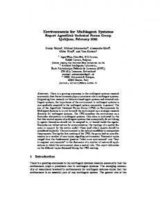
resource in R a replacement can be found, the auctioneer tells the requesting agent a that it may discard the corresponding skill(s). The replacing resources are marked as goals for the providing agents, and become additional ‘initial’ resources for agent a. If not all resources can be replaced, the request is retried after completion of all other requests. This process is repeated until none of the auctions has been successful. Algorithm 1 describes this auction algorithm in more detail. Algorithm 1 ground plan merging ( A ) 1. retrieve requests from all agents A 2. repeat 2.1. while some requests left do 2.1.1. get the request with the highest priority 2.1.2. ask the requesting agent a for the required resources R 2.1.3. for each a0 ∈ A, a0 6= a do ask a0 for free resources similar to resources in R add these to R0 2.1.4. let R00 ⊆ R0 be the cheapest set, s.t. R00 ≈ R 2.1.5. if successful, i.e., R00 ≈ R then actually replace R by R00 for agent a mark all resources from R00 as goals for their respective delivering agent 2.1.6. if failed then store this failed request in a secondary storage 2.2. restore all failed requests until there has not been a successful replacement In the following we continue Example 5 by showing the effect of plan merging on the plans of the agents. Example 6 Running ground plan merging for agents a1 and a2 , as described in Example 5, results in the following plan modifications. Each agent returns a set of requests to the auctioneer. For a1 this is at most {(drive C, 1), (drive D, 2), (drive E, 3), (travel, 4)}, and for a2 {(drive B, 1), (drive C, 1), (drive D, 2), (travel1 , 1), (travel2 , 3)}. Each request consists of a resource and a number indicating the potential cost reduction. In this example each skill has costs one. The requests are put in a priority queue based on this cost reduction. Subsequently, the one with the highest potential cost reduction is selected, that is (travel, 4) by a1 , and the required resource(s) are determined: {p(3, E, [7, ∞])}. Unfortunately, agent a2 does not have this resource in its free resource set. So this request is stored in the secondary storage. Most of the other requests do not lead to a success either. The only request that allows for plan optimization is (drive D, 2) by agent a2 . The required resource for this request is {ride(C, D, 2, [5, 5])} and a1 happens to have this resource available. This resource is then used in the plan of agent a2 to replace the similar resource produced by drive D, and so two skills can be removed from this plan: drive D and therefore also drive C, as it then does not produce any product anymore that is used by another skill or marked as a goal. The resource ride(C, D, 2, [5, 5]) is marked as a goal for agent a1 , resulting in the merged plan depicted in Figure 4. The ground plan merging algorithm is an any-time algorithm, because it can be stopped at any moment. If the algorithm is stopped, it will still return an improved set of agent plans, because this algorithm used a greedy policy, i.e., dealing with the requests with the largest potential cost reduction first. In the next section we describe a more flexible version of such an any-time merging algorithm.

3.2

Flexible plan merging

The ground plan merging algorithm can be too restrictive, because only resources that are similar, are accepted as a replacement. In general, a replacement should be an instantiation of the same 21

ride(C, D, 1, [5, 5]) p(2, D, [6, ∞])

p(3, E, [7, ∞])

travel2

ride(D, E, 1, [6, 6])

travel p(3, D, [1, ∞])

p(2, C, [2, ∞])

ride(C, D, 2, [5, 5])

taxi(2, E, [7, ∞]) ride(D, E, 2, [6, 6])

drive E

ride(A, B, 1, [3, 3]) p(1, B, [4, ∞])

ride(C, D, 2, [5, 5]) taxi(2, D, [6, ∞]) travel1 drive D p(1, A, [1, ∞]) ride(A, B, 2, [3, 3]) taxi(1, B, [4, ∞])

drive B

ride(F, C, 2, [4, 4])taxi(2, C, [5, ∞])

drive C

taxi(2, F, [4, ∞])

taxi(1, A, [3, ∞])

Figure 4: The merged plan for agent a2 (left) and agent a1 (right). resource scheme and satisfy the same constraints. These constraints are (i) the constraints of the skill or goal that uses this resource, and (ii) indirectly constraints on subsequent skills and the goal constraints. We first give an example of a situation in which the ground plan merging algorithm does not give the desired result. Example 7 In Example 6 we have seen how a resource can be exchanged in a ground plan to improve the joint efficiency. Suppose now that the initial resources of a1 are {taxi(2, F, [3, ∞]), p(3, D, [1, ∞])} instead of {taxi(2, F, [4, ∞]), p(3, D, [1, ∞])}. A planner now might come up with a plan where every resource is produced one time unit earlier. Intuitively, it is clear that a similar exchange would still be possible. However, the original plan merging algorithm is too restrictive to discover this possibility, because the requested resource {ride(C, D, 2, [5, 5])} by agent a2 and the free resource {ride(C, D, 2, [4, 4])} by agent a1 are not similar. In the flexible plan merging algorithm, a request is not specified by a set of resources, but by a set of resource schemes together with a set of constraints on the values of the attributes of these schemes. All constraints on the requested resource schemes are extracted from the services involved in the plan by the requesting agent. Each agent returns only those free resources that satisfy at least one of the resource schemes, such that the set of constraints is satisfiable. It is the task of the auctioneer to find a combination of those returned resources that satisfies both the set of resource schemes and all constraints (preferably with minimal costs). In general, the complexity of the flexible plan merging algorithm (Algorithm 2) that solves this problem is exponential for the auctioneer, but in practice the time complexity is usually limited (see Section 3.3).8 Algorithm 2 flexible plan merging ( A ) 8 Unfortunately, in general, when the constraints range over all resource schemes and resources satisfy any of the resource schemes, this problem is NP-hard.

22

1. retrieve requests from all agents A 2. repeat 2.1. while some requests left do 2.1.1. extract the request with the highest priority 2.1.2. let a be the agent placing this request for skill s 2.1.3. using function get constraints( a, s ) (see Algorithm 3) get the required resource schemes and the constraints C from agent a 2.1.4. for each a0 ∈ A, a0 6= a do return all free resources r of a0 , such that ∃rs ∈ RS : r |= rs and C(r) is satisfiable, to the auctioneer, storing it in the set R0 2.1.5. R00 = the cheapest combination R00 ⊆ R0 such that R00 |= RS and C(R00 ) is satisfiable 2.1.6. if successful then replace RS by R00 and update agent a’s plan; mark all resources from R00 as goals for their respective delivering agent 2.1.7. if failed then store this failed request in a secondary storage 2.2. restore all failed requests until there has not been a successful replacement In Step 2.1.3 of Algorithm 2, the constraints on the requested resources are determined. This procedure is somewhat complicated, because a requested resource r may be used by a skill s having constraints on it. The skill s may produce resources R that due to range-restrictedness (see Definition 6), are functionally dependent on this resource r. These resources R, in turn, may be used by other skills or as a goal, again introducing constraints on r (indirectly). The set of all constraints C on the requested resources can be derived as follows. For an agent a, a set of requested resources Rx , the corresponding set of resource schemes RSx , a set of resources R from the plan of a, and a set of constraints C on R, we define a recursive function, get constraints on(a, Rx , RSx , R, C). This function creates a resource scheme RS corresponding to R, such that the attributes of RS are expressed as a function of the attributes of RSx , and returns all constraints on RSx , including the constraints C. Let RI denote the set of initial (ground) resources. In case R ⊆ Rx ∪ RI , the set of constraints C already is of the correct type (on RSx and some constants) and may be returned, and the attributes of R are also correct (either constant or a function of attributes of Rx ). If there are resources in R that are not ground and not in Rx , then the attributes of the resources R need to be expressed as a function of the attributes of Rx ∪ RI . For each resource r ∈ R that is not in Rx ∪ RI , there is a skill s that produces r. The attributes of r are functionally dependent on the input resources of s. A recursive call of get constraints on the input resources of s, ensures that the attributes of the input resources, and thus the attributes of r can be expressed as a function of the attributes of Rx ∪ RI , and so can the constraints C. The get constraints on algorithm (see Algorithm 3) is initiated with the set of free resources and the goal constraints. Algorithm 3 get constraints ( a, s ) 1. let Rx be the set of output resources of s to be replaced 2. let RSx ⊆ out(s) be the set of resource schemes representing Rx 3. let R be the set of free resources of the plan of agent a 4. let C be the set of goal constraints to be satisfied by agent a 5. let Scomp be the (global) set of completed skills, initially ∅ 6. return RSx and the constraints on RSx , using the function: get constraints on ( a, Rx , RSx , R, C ) 1. let CB be ∅

23

2. of 3. 4. 5.

6.

7. 8. 9.

determine the set of skills S producing R by tracing one step backwards in the plan graph agent a let S 0 = S − Scomp be the skills that have not been dealt with add all skills from S 0 to Scomp for each s ∈ S 0 do 5.1. determine the set R0 of input resources of s 5.2. get constraints on RSx , given output resources R0 and constraints on s (get constraints on ( a, Rx , RSx , R0 , Cs )) 5.3. add these constraints to the constraint base CB for each resource r ∈ (R − Rx ) do express the attributes of r in terms of the attributes of the input resources of the skill s that produces r in the plan of agent a evaluate the constraints C on the attributes of R add them to the constraint base CB return CB

We now show how the constraints introduced in Example 7 are derived. Example 8 The set of resource schemes needed for the request (drive D, 2) of agent a2 is {ride(C, D, c, [t, t])} and the constraint base is {c ≥ 1, 2 ≤ t, t ≤ 7}. The first two constraints come directly from the constraints of the drive skill. The third constraint is a result of an evaluation of the goal constraint combined with the functional dependency of the goal p(2, D, [t1 , t2 ]) on the ride resource: t1 = t + 1 ≤ 8. It is easy to see that the resource ride(C, D, 2, 4) matches these constraints.

3.3

Complexity analysis

In this section we analyze the time complexity of both plan merging algorithms. We start by giving the complexity analysis of flexible plan merging, because, as we will see, ground plan merging is a special case of flexible plan merging. First, however, we make some assumptions. Let n be the number of skills in the joint plan of all agents. We suppose there is a constant c ≥ 1 such that for all skills s holds that |in(s)|, |out(s)| ≤ c, and |Cs | ≤ c, and thus (because a request is related to the removal of one skill) for all requests G also |G| ≤ c. Then, because the number of resources related to a skill is bounded by this constant c, we may conclude that the number of resources is O(n), as is the time complexity of one traversal through the plan graph. Proposition 5 Given a set of skills S, the worst-case time complexity of the flexible plan merging algorithm is O(n2+cS ), where cS = maxs∈S {|in(s)| , |out(s)| , |Cs |}. Proof 6 In Step 1 of Algorithm 2 the requests of the agents are collected and the cost-reductions determined. This can be done by one traversal of the plan of the agent, and thus takes O(n) time. The repeat loop (Step 2) is stopped once there is no change. A change is the removal of a skill. So this loop, in the worst case, is traversed O(n) times. In the worst case, the while-loop (Step 2.1) inside this repeat-loop may be executed O(n) times as well, since there are at most O(n) requests. We discuss the steps of this while-loop that, at first sight, take more than constant time: Finding the request with the highest priority can be done, e.g., by a priority queue, taking aggregated O(1) time. Step 2.1.3 determines the constraints on the request.9 This is Algorithm 3. Because of the set of completed skills, each skill is considered only once, so, given that the functions can be evaluated in constant time, this step takes O(n) time. Step 2.1.4 takes O(n) time as well, given that constraints can be evaluated in constant time, because at most O(n) free resources are considered. In Step 2.1.5, in the worst case, all combinations of size cS from the set
of O(n) resources need to be considered, taking O( ncS ) = O(ncS ) time steps. Finally, Step 2.1.6 may take O(n) time, because in some cases a whole sub-tree may be deleted. 9 For

a detailed description and analysis of priority queues see, e.g., Cormen et al. [4].

24

All other steps take constant time, as can be easily seen. The time complexity of the flexible plan merging algorithm is O(n) for the repeat-loop, times O(n) for the while-loop, times O(ncS ) for the contents of the while loop, resulting in a total time complexity of O(n2+cS ). Proposition 6 The ground plan merging algorithm has worst-case time complexity of O(n3 ). Proof 7 We use the proof of Proposition 5. It can be easily seen that the complexity of the steps of ground plan merging is equal to the equivalent steps of flexible plan merging. There is, however, one important difference: Step 2.1.5 in flexible plan merging of O(nc ) is related to Step 2.1.4 of ground plan merging of O(n). Therefore the total time complexity of ground plan merging is O(n3 ). The time-complexity of flexible plan merging is caused by the dependencies between the resource schemes. For example, it can be seen that, if (i) for each resource scheme rs, the set of constraints on rs only involves rs, and (ii) the set of resources that satisfies rs and Crs is disjoint from sets of resources satisfying other resource schemes, then the selection of the cheapest combination can be done in linear time, like in ground plan merging. Proposition 7 bounds this dependency by a constant, depending on the set of goal schemes and the set of skills used. First, we need to define a so-called dependency constant for a set of constraints on a set of resource schemes. We use res(C) = RS to denote the set of resource schemes whose attributes occur in the constraints in C (so all attributes occurring in C belong to RS). Definition 23 For a set of constraints C on a set of resource schemes RS, the dependency constant, dC is defined as follows: If there exists a partition C1 ∪ . . . ∪ Cm of C such that 1. res(C1 ) ∪ . . . ∪ res(Cm ) is a partition of RS, and 2. there is no resource r that for i 6= j satisfies both Ci and an rsi ∈ res(Ci ), as well as Cj and an rsj ∈ res(Cj ), then we define the dependency constant dC to be the size of the largest part of the partition of resource schemes, i.e., dC = max1≤i≤m |res(Ci )|. Proposition 7 Given the set of all goal schemes GC and the set of all skills S. If  d = max maxs∈S dCs , max(G,C)∈GC dC then the time complexity of flexible plan merging is O(n2+d ). Proof 8 By definition of d, we know that the resource schemes can be partitioned into sets of at most size d. Choosing a combination of resources with minimal costs that satisfies such a set of resource schemes costs, in the worst case, O((c · n)d ) time steps, where 0 ≤ c ≤ 1. If for P all k sets of resource schemes, each set i is possibly satisfied by at most O(ci · n) resources, with ci = 1, then we know that the total time complexity of the Step 2.1.5 in flexible plan merging is P d d O((c · n) ) = O(n ). By the proof of Proposition 5, the result follows. i 1≤i≤k The following example illustrates these properties. Example 9 In our model of the taxi company domain, all skills have at most two input and two output resource schemes. So we have c = 2, and therefore the plan merging algorithm has time complexity O(n4 ). Using Proposition 7, we derive the following: In one case (the travel skill) we have a skill constraint with d = 2 (see Definition 23). If we further require that all goals (G, C) are modeled such that dC ≤ 2, in other words, no goals may be specified so vague that one resource may satisfy more than two goals, this also leads to a time complexity of O(n4 ).

25

4

Discussion

We proposed a formalism in which we are able to express all kinds of constraints on all kinds of attributes. Our plan merging algorithm deals with these constraints and reallocates resources to improve efficiency in a distributed way. Our algorithm is an approximation, using a greedy heuristic, and can be stopped at any time. We also give some restrictions on the problem that allows a very efficient plan merging. Furthermore, we deal with private knowledge of the agents. Dealing with conflicts between agents, insincere agents, interleaving planning and execution, and replanning is future work (see Section 4.3). This work is strongly related to other work in both the multi-agent community, especially multi-agent planning and multi-agent problem solving, and the computational logic community. In this section we first relate our work on plan merging to other plan merging methods. In Section 4.2 we mention some other logics that are used for planning and we show how they are different from our approach. We conclude with a discussion on future work.

4.1

Relation with other plan merging methods

In the beginning of the eighties Rosenschein [24] proposed ways to deal with conflicts between agents that can be resolved by synchronizing the execution of their plans. He showed what to communicate to resolve undesired interactions, so-called conflicts. He did not show, however, how to improve the efficiency of plans by cooperation, nor how to cope with quantitative resources like capacity or costs. In our framework we have not paid much attention to resolution of conflicts. However, we assume an initial distribution of all available resources. This resolves most of the conflicts, since an agent may not sell a resource it needs itself. The work of Georgeff [15, 16] on multi agent planning was also not to improve a set of plans, but to ensure that two or more plans do not conflict. In [16] Georgeff defines a so-called process model to formalize the actions open to an agent. Part of a process model are the correctness conditions, defined over the state of the world, that must be valid before execution of the plan may succeed. Two agents can help each other by changing the state of the world in such a way that the correctness conditions of the other agent become satisfied. Of course, changing the state of the world may help one agent, but it may also interfere with another agent’s current plan. That is, one agent may change the state of the world in such a way that the correctness conditions of another agent become invalid. In our current work we assume that agents already have correct plans available that realize the set of goals before they agree to cooperate to optimize their plans. The notion of correctness conditions could be helpful when we incorporate situations where cooperation between agents is needed to realize the set of goals. Logic and planning were combined by Stuart [26] to find out whether individual plans can be synchronized. Using Propositional Temporal Logic, constraints are generated from plans to specify the feasible states of the environment. These constraints are given to a theorem prover to generate sequences of communication acts that guarantee that no event will fail. Just as Georgeff, Stuart focuses on the resolution of conflicts, and not on potential positive relations between plans. Our framework can also be compared with the PGP (Partial Global Plan) framework described by Durfee et al. ([9, 8]) and Decker and Lesser ([7]). In this PGP-framework and its extension GPGP, agents are allowed to cooperate by exchanging parts of their local plans to develop common plans. The main difference with our approach to cooperation is that in our framework exchanging parts of local plans is more involved, since exchanging parts of a plan will usually change not only the agent commitment structure but will also affect the structure of the local plans involved. Plan merging was also studied by Von Martial [27, 28]. He considers several types of relations between plans, divided into conflicts and positive relations. Plans are represented hierarchically and need to be exchanged among the agents to determine such relations. If possible, relations are solved or exploited at top-level. If this is not possible, a refinement of the plans is made and the process is repeated. For each specific type of plan relationship a different solution is presented. Our plan merging algorithm is applied at a low-level representation of the plan, not needing any domain specific information, nor communicating the complete plan of one agent to another. 26

Clement and Durfee [2, 3] describe an interleaved planning process, where different agents jointly construct a plan to establish a set of goals. They use the class of planners called Hierarchical Task Network (HTN) planners like Von Martial’s hierarchical plans. To avoid unnecessary backtracking, the agents must recognize whether their plans interfere before the plans are fully refined. Clement and Durfee derive the so-called plan summary information from the hierarchical plan operators. Using this summary information, they can reason about possible interactions between different agents before the individual plans are completely specified. It would be interesting to analyze how in a similar way summary information can be derived and used to recognize opportunities to optimize plans of individual agents. Both to improve efficiency and to resolve conflicts, restrictions may be introduced on individual plans to ensure efficient merging. This work by Yang [29] and Foulser [14] is also useable to merge alternative plans to reach the same goal. Furthermore, some approximation algorithms for plan merging are described by the same authors. They do not, however, deal with costs, quantitative constraints on resource attributes, and their algorithms are not distributed. Finally, we would like to mention the work on plan merging by Ephrati and Rosenschein [10, 11, 12]. Their approach resembles our work the most, because they also developed a distributed polynomial algorithm to improve social welfare (i.e., the sum of the benefits of all agents). Through a process of group constraint aggregation, agents incrementally construct an improved plan by voting about joint actions. They even propose algorithms to deal with insincere agents and to interleave planning,coordination, and execution. But, neither they do pay attention to dealing with numerical constraints, time, and costs. The main difference between their approach and ours, is that our algorithms can be formulated by a resource logic, while theirs use a description of the state of the world by propositions, like in STRIPS, as is discussed in the next section.

4.2

Relation with other planning logics

Several planning logics have been proposed in the literature that are more or less close to the one developed in this paper. The most popular of these are STRIPS that is based on first-order logic [13], and extensions of it like PDDL [21] and Functional STRIPS [1]. STRIPS resembles our formalism with respect to the fact that for each operator explicitly is stated which atomic facts are to be deleted from the current state and which have to be added to create the new state. The atomic facts in the STRIPS formalism are, so to speak, the resources of the resource-skill formalism. This enables embedding STRIPS in the latter. However, unlike our formalism, STRIPS is not suited to directly handle parallel actions, to deal with quantities like capacities, distances, costs, and time, and to model cooperation between agents. The resource-skill formalism has also a strong resemblance to the revision specification programs developed by Marek and Truszcynski [19]. In these programs rules not only are used to create other atoms or resources but also to remove them given the presence of some input atoms and the absence of others. Although their formalism uses Horn-like rules, skills can be simulated by revision specification programs. The reverse way is also possible, i.e., modeling revision processes using the resource-skill formalism. This result is interesting since it opens the door to applying logic programming techniques to our formalism. An important difference of our work and the work by Marek and Truszcynski, is the fact that the resource-skill formalism deals with constraints and services as the composition of skills. Furthermore, we developed plan merging algorithms for which our plan representation is very suited. Another planning logic that is very close to ours is the one developed by Masseron et al. [20]. One important difference is the fact that in their formalism it is possible to include nondeterministic actions, i.e., actions with an outcome that is uncertain albeit limited to a set of given outcomes. On the other hand, our formalism can handle constraints, whereas the planning logic of Masseron et al. does not. For their variant, they constructed a correct and complete embedding in a fragment of linear logic. Linear logic, invented and developed by Girard (see, e.g., [18]) is a so-called substructural logic that emerges if structural rules such as weakening and contraction are discarded. Since resources, 27

be it in the sense of our formalism or that of Masseron et al., can be only used once (no absorption), linear logic can be considered a good candidate as a planning logic. So it seems quite natural to study the relationship between planning and linear logic. However, the fragment of linear logic used for the embedding, is very restricted. It turns out that skills and resources have to be translated as a linear theory, using only one linear logical connective (multiplicative conjunction) in the deterministic case, and two (multiplicative conjunction and additive disjunction) in the nondeterministic one. In their paper, Masseron et al. do not touch the problem of plan merging. In our opinion our presentation of the planning formalism is better suited to study the operational behavior of planning. Our choice of describing the operational semantics of plans by a transition system (cf. Structural Operational Semantics as introduced by Plotkin [23]) underlines this idea. We also have given evidence of the usefulness of our planning formalism to model plan merging.

4.3

Future work

Many applications induce additional requirements on our formalism or algorithms. For example, we would like to develop a mechanism to solve conflicts between agents, such as both agents requiring the same resource. Until now, we assumed all resources have initially been distributed over all agents. This is not realistic in all circumstances, e.g., in cases where agents have to share (scarce) resources. Therefore, we would like to adapt our algorithms to this kind of situations. This could be done, for instance, by incorporating auctioning mechanisms in which agents have to make bids for allocating resources. Another important issue for future research is the interleaving of planning and execution. Our algorithms are developed from the point of view that agents already have made up their plans before cooperating with other agents. This is a very static view of reality. It would be much more realistic to interleave the process of planning and cooperation, for it is often during planning that the necessity of cooperation seems to become inevitable. The last point is also of importance in the light of replanning. Replanning is necessary when circumstances are not as expected beforehand due to unforeseen events. For instance, a transportation agent might have to change his route on the way because of a severe traffic jam. So, planning has to be a dynamic process. From this observations it is clear that we have to direct our research to planning as well. Since, from a computational point of view, planning is a difficult problem, we have to develop approximation techniques for this problem. There are many other directions in which our formalism or our algorithms could be extended. To mention two of these: how to cope with systems in which not all agents are to be trusted (insincere agents), how do we model the various kinds of relationships that are possible between agents (sociological agents). Finally, we are about to test our algorithms with data from public transportation. In this way we hope to substantiate our claim that our cooperation algorithms may improve plan efficiency in a substantial way.

Acknowledgements We like to thank Roman van der Krogt for his comments on this paper and for his help with the formalism and the algorithms. Furthermore, we greatly appreciate the detailed comments of the reviewers that really helped us to improve this paper.

References [1] Blai Bonet and H´ector Geffner. Functional strips: A more general language for planning and problem solving. In Proceedings of the Logic-Based AI Workshop, 1999.

28

[2] Bradley J. Clement and Edmund H. Durfee. Theory for coordinating concurrent hierarchical planning agents using summary information. In Proceedings of the Sixteenth National Conference on Artificial Intelligence (AAAI-99), pages 495–502, 1999. [3] Bradley J. Clement and Edmund H. Durfee. Top-down search for coordinating the hierarchical plans of multiple agents. In Proceedings of the Third International Conference on Autonomous Agents (Agents-99), pages 252–259, 1999. [4] T.H. Cormen, C.E. Leiserson, and R.L. Rivest. Press/McGraw-Hill, 1990.

Introduction to algorithms.

MIT

[5] Mathijs M. de Weerdt, Andr´e Bos, Hans Tonino, and Cees Witteveen. Fusion of plans in a framework with constraints. In Proceedings of the ISCS Conference on Intelligent Systems and Applications (ISA-00), pages 393–399, 2000. [6] Mathijs M. de Weerdt, Andr´e Bos, J.F.M. Tonino, and Cees Witteveen. A resource logic for multi-agent plan merging. Annals of Mathematics and Artificial Intelligence, special issue on Computational Logic on Multi-Agent Systems, 37(1–2):93–130, Januari 2003. [7] Keith S. Decker and Victor R. Lesser. Designing a family of coordination algorithms. In Proceedings of the 13th International Workshop on Distributed Artificial Intelligence, pages 65–84, Lake Quinalt, Washington, 1994. [8] E. H. Durfee. Coordination of Distributed Problem Solvers. Kluwer, 1988. [9] E. H. Durfee and V.R. Lesser. Using partial global plans to coordinate distributed problem solvers. In Proceedings of the Tenth International Joint Conference on Artificial Intelligence (IJCAI-87), pages 875–883, Milan, Italy, 1987. [10] E. Ephrati and J. S. Rosenschein. Multi-agent planning as a dynamic search for social consensus. In Proceedings of the Thirteenth International Joint Conference on Artificial Intelligence (IJCAI-93), pages 423–429, Chamb´ery, France, 1993. [11] Eithan Ephrati and Jeffrey S. Rosenschein. Multi-agent planning as the process of merging distributed sub-plans. In Proceedings of The Twelfth International Workshop on Distributed Artificial Intelligence, pages 115–129, May 1993. [12] Eithan Ephrati and Jeffrey S. Rosenschein. Divide and conquer in multi–agent planning. In Proceedings of the Twelfth National Conference on Artificial Intelligence (AAAI-94), pages 375–380, Seattle, WA, 1994. [13] R. E. Fikes and N. Nilsson. STRIPS: A new approach to the application of theorem proving to problem solving. Artificial Intelligence, 5(2):189–208, 1971. [14] D.E. Foulser, Ming Li, and Qiang Yang. Theory and algorithms for plan merging. Artificial Intelligence Journal, 57(2–3):143–182, 1992. [15] Michael Georgeff. Communication and interaction in multi-agent planning. In Proceedings of the Third National Conference on Artificial Intelligence (AAAI-83), pages 125–129, Washington, D.C., August 1983. See also [17]. [16] Michael Georgeff. A theory of action for multiagent planning. In Proceedings of the Fourth National Conference on Artificial Intelligence (AAAI-84), pages 121–125, Austin, TX, August 1984. (Also published in Readings in Distributed Artificial Intelligence, Alan H. Bond and Les Gasser, editors, pages 205–209, Morgan Kaufmann, 1988.). [17] Michael Georgeff. Communication and interaction in multi-agent planning. In A. Bond and L. Gasser, editors, Readings in Artificial Intelligence, pages 200–204. Morgan Kaufmann Publishers, San Mateo, CA, 1988. 29

[18] J.-Y. Girard. Linear logic. Theoretical Computer Science, 50:1–102, 1987. [19] V.W. Marek and M. Truszczynski. Revision specifications by means of programs. In C. MacNish et.al., editor, European Workshop, JELIA’94, York, UK, September 1994, Proceedings, Lecture Notes in Artificial Intelligence 838, pages 122–136, Berlin, 1994. Springer-Verlag. [20] M. Masseron. Generating plans in linear logic. Theoretical Computer Science, 113(2):349–370, 1993. [21] D. McDermott. PDDL – the planning domain definition language. Technical Report TR-98003, Yale Center for Computational Vision and Control, October 1998. [22] Bart-Jan Moree, Andr´e Bos, Hans Tonino, and Cees Witteveen. Cooperation by iterated plan revision. In Proceedings of the Fourth International Conference on Multi-Agent Systems (ICMAS-00), 2000. [23] G. Plotkin. An operational semantics for CSP. In D. Bjørner, editor, Proceedings IFIP TC 2 Working Conference: Formal Description of Programming Concepts – II, pages 199–223, Amsterdam, 1983. North-Holland. [24] Jeffrey S. Rosenschein. Synchronization of multi-agent plans. In Proceedings of the Second National Conference on Artificial Intelligence (AAAI-82), pages 115–119, Pittsburgh, PA, August 1982. (Also published in Readings in Distributed Artificial Intelligence, Alan H. Bond and Les Gasser, editors, pages 187–191, Morgan Kaufmann, 1988.). [25] O. Shehory and S. Kraus. Methods for task allocation via agent coalition formation. Artificial Intelligence, 101(1–2):165–200, May 1998. [26] Christopher J. Stuart. An implementation of a multi-agent plan synchronizer. In Proceedings of the Ninth International Joint Conference on Artificial Intelligence (IJCAI-85), pages 1031– 1033, Los Angeles, CA, August 1985. (Also published in Readings in Distributed Artificial Intelligence, Alan H. Bond and Les Gasser, editors, pages 216–219, Morgan Kaufmann, 1988.). [27] Frank von Martial. Interactions among autonomous planning agents. In Y. Demazeau and J.P. M¨ uller, editors, Decentralized AI Decentralized AI — Proceedings of the First European Workshop on Modelling Autonomous Agents in a Multi-Agent World (MAAMAW-89), pages 105–119. North Holland, 1990. [28] Frank von Martial. Coordinating Plans of Autonomous Agents. Springer-Verlag, Berlin, 1992. Lecture Notes in Artificial Intelligence no. 610. [29] Qiang Yang, Dana S. Nau, and James Hendler. Merging separately generated plans with restricted interactions. Computational Intelligence, 8(4), November 1992.

30