Theory and Algorithms for Plan Merging - CiteSeerX

Theory and Algorithms for Plan Merging David E. Foulser



Ming Li

y

Qiang Yang

z

Abstract

Merging operators in a plan can yield signi cant savings in the cost to execute a plan. This paper provides a formal theory for plan merging and presents both optimal and ecient heuristic algorithms for nding minimum-cost merged plans. The optimal plan-merging algorithm applies a dynamic programming method to handle multiple linear plans and is extended to partially ordered plans in a novel way. Furthermore, with worst and average case complexity analysis and empirical tests, we demonstrate that ecient and well-behaved approximation algorithms are applicable for optimizing plans with large sizes.

Silicon Graphics Computer Systems, M/S 7U-550, 2011 N. Shoreline Blvd., Mountain View, CA 94039, USA. Supported in part by Oce of Naval Research grant N00014-86-J-1906 and by NIH Grant R01 LM05044 from the National Library of Medicine. y Department of Computer Science, University of Waterloo. Waterloo, Ontario, Canada, N2L 3G1. Supported in part by NSERC operating grants OGP0036747 and OGP0046506. z Department of Computer Science, University of Waterloo. Waterloo, Ontario, Canada, N2L 3G1. Supported in part by NSERC operating grant OGP0089686 and an ITRC grant. 

1

2

1 Introduction

1.1 The Plan Merging Problem

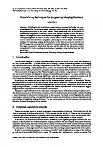
The value of helpful or positive interactions among the dierent parts of plans was recognized early in AI planning research [13, 16, 18]. A helpful goal interaction occurs in a plan, or among several plans, if certain portions of the plan can be modi ed to improve its quality. An important type of helpful goal interaction occurs when certain operators in a plan can be grouped, or merged, together in such a way as to make the resulting plan more ecient to execute. This happens often in domains where redundant setup and restore operations can be eliminated in the execution of consecutive tasks and where redundant journeys can be eliminated by fetching multiple objects at once. Consider the following description given by Wilensky [17]. John was planning to go camping for a week. He went to the supermarket to buy a week's worth of groceries. The main character in this example, John, had a set of subgoals to achieve, each subgoal being to buy food for a meal during the camping week. However, instead of making several shopping trips separately for each individual meal, John was able to merge the plans for the subgoals, and achieve them simultaneously with a single trip to the market. The resultant merged plan is more ecient to execute than the separate ones. Merging actions for reducing plan costs, as demonstrated above , is typical of the kind of optimization task people do for general transportation problems. For example, suppose that cargo items A and B both need delivered from location L1 to location L2 by planes. If the two delivery goals are planned separately, then two airplanes would be required for both A and B. For each item, a separate loading and unloading operation are needed. However, if A and B t into one plane, then combining the two sub-plans can produce a more ecient overall plan for both goals. This merged plan requires one combined loading and unloading operation for A and B, as well as a single ying operation. The result is a plan that is considerably cheaper than the original ones. Plan merging is equally important for minimizing the costs of robot task plans. As an example, consider a blocks world problem with variable-sized blocks. To pick up one block of a certain size, the robot arm has to mount a gripper of an appropriate size. Suppose that only one robot arm exists, and in order to grab a block of a dierent size, the robot has to unmount the current gripper and mount the gripper with the new size. In this case, it is more ecient to group block stacking operations that use the same type of grippers. In the example shown in Figure 1, the blocks are of two dierent sizes. Suppose that the robot can use two dierent grippers of type A and B to pick up a corresponding type of block. Then a minimal cost way for achieving the goal would be to move A1 and A2 to the table together, then move B1 and B2 to the the top of A1 and A2. This plan saves two gripper changing operations as compared with moving A's and B 's interleavingly.

3 Initial

Goal

A1

A2

B1

B2

B1

B2

A1

A2

Figure 1: A blocks world where blocks are of dierent sizes. The blocks world problem is illustrative of the role of operator merging in robotic assembly domains. Identical plan merging issues also arise in the domain of automated manufacturing where process plans for metal-cutting [6], set-up operations [4] and tool-approach directions [10] need to be optimized. Similarly, in the area of query optimization in database systems [15], as well as domains having multiple agents [2, 12], operator merging in multiple plans seems inevitable.

1.2 Previous Work

Sacerdoti's NOAH [13] system is one of the rst planners to explicitly seek opportunities for plan merging. It relies on its set of Critics to handle possible interactions among the dierent parts a plan. Three critics are introduced for the purpose of improving the quality of plans, including \eliminate redundant preconditions," \use existing objects" and \optimize disjuncts." For example, the \eliminate redundant preconditions" critic can be considered as merging two or more operators that are used to achieve the same preconditions, as long as no precedence relation in the plan is violated. Wilkins' SIPE [18] and Tate's NONLIN [16] are other planning systems that have relatively more advanced capabilities in operator merging. For example, they are able to recognize that a goal is achievable by another operator in the current plan. In such situations, it will impose constraints on orderings and variable bindings so that the operator is used to achieve it. This process, known as phantomization of a goal, is also used in the plan reuse framework of Kambhampati's plan reuse framework for reducing plan cost [?]. At a meta-planning level, Wilensky [17] considers dierent types of positive goal relationships, in the context of cognitive modeling of human problem solving. In contrast to the above domain-independent approaches to planning, Hayes [4] proposed a domain-dependent method for plan merging in machining domains. In her Machinist system, a greedy algorithm is implemented and compared with human machinists in terms of the quality of the plans produced. It was shown that it can out-perform an experienced human process planner in many instances. As an intermediate approach that falls between domain-independent and domain-dependent extremes, Yang, Nau and Hendler [11] proposed a limited-interaction approach to planning,

4 taking into consideration operator merging as one type of interactions allowed. In recognizing the complexity of the general problem, they imposed certain restrictions that work well for a number of domains. An interesting feature of their system is that they considered the case where there is more than one alternate plan for each goal, and proposed a branch and bound algorithm for selecting the plans that can be merged optimally from a set of alternative choices. These previous research have had successes in various practical domains. But the understanding of plan merging has largely remained at a qualitative level. Most existing systems have adopted some heuristic methods for encouraging plan merging, but little has been known about the condition under which plans may be merged, the computational complexities of optimal and approximate algorithms for plan merging, as well as the quality of the merged plans that the approximation algorithms produce. This lack of knowledge is partly due to the fact that the majority of planning research so far has concentrated on methods for dealing with negative relationship among goals and plans, such as goal con ict and resource competitions. As a consequence, formal theories are appearing on methods for constructing sound and complete planners[1], for eciently resolving con icts [19, 1], for reusing past planning experiences[5], and for building \good" abstraction hierarchies [7, 21] for improving problem-solving eciency. A common theme of these research has been on nding a solution that works. In contrast, this paper attempts to address the issues of nding solutions with optimal or \good" quality.

1.3 Overview

The purpose of this paper is to develop a computational theory on plan mering. This theory will attempt to address the following issues: 1. What are the conditions under which operators in a plan can be merged? 2. What is the computational complexity of optimal plan mering? 3. What are the optimal algorithms for plan merging? When are these algorithms feasible in practice? 4. Where the optimal algorithms are infeasible to apply, what are the approximation algorithms that perform fast? What are the worst and average-case complexities of these algorithms? Our approach to addressing the above questions is to combine formal methods developed in Arti cial Intelligence and computational techniques from Operations Research (OR). In particular, we rst propose a formalization of plan merging using the STRIPS operator de nitions. Based on the formalization, we present a dynamic programming algorithm for determining the optimal solution by reducing the problem to the shortest common supersequence problem, a variant of the longest common subsequence problem, and apply several

5 known results from that area. While the dynamic programming algorithm has traditionally formulated for inputs corresponding to matrices of symbols, AI planning has been concerned about plans represented as partially ordered operator sets. To bridge the two dierent elds, we also extend the dynamic programming method to handling partially ordered plans in a novel way. One drawback of the dynamic programming method is that it becomes computationally infeasible for problems of larger sizes. While we are able to phrase an optimal algorithm for general purpose, domain-independent plan merging, its run time requirements may be prohibitive for inputs of practical sizes. To make the planning problem more tractable, most existing systems that consider helpful interactions employ certain kinds of greedy algorithms for plan merging [4, 13, 16, 18]. Thus, we also describe four approximation algorithms for merging plans, and analyze the qualities of their outputs in average cases. The approximation algorithms all have linear time complexity in the number of operators of the input plan. Finally, we present a set of empirical results comparing the quality of the plans produced by the optimal and approximation algorithms under various conditions. The remainder of the paper has the following organization. Section 2 gives a formal description of plan merging. Section 3 presents the optimal algorithm for merging linearly ordered plans. Section 4 extends the traditional dynamic programming algorithm to partially ordered plans as well. Section 5 develops four approximation plan merging algorithms and analyzes their behavior. Section 6 presents experimental results for the four heuristic methods. Conclusions are stated in section 7.

2 Formal Description of the Problem

2.1 A Formal De nition of Operator Merging

Given a set of goals to be achieved, a plan  is a partially ordered set of operators, where each operator  is represented by preconditions P and eects E, which for the sake of simplicity are assumed to be sets of literals (positive or negative atomic sentences). No operator's preconditions or eects can contain both a literal and its negation. A plan  may be represented as a graph  = (O; B ) where the vertices O are the set of operators in  and the edges B are the set of precedence relations in . It is also assumed that two special operators exist in every plan  that represent the initial and goal states in . The initial state operator I precedes all other operators in , and the goal state operator G is preceded by all other operators. I has an empty set of preconditions, and has as its eects the set of initial conditions. Likewise, the goal operator G has an empty set of eects, and has as its preconditions the goal conditions to be achieved. In a least-commitment plan, there is usually a set of constraints on the binding of variables, known as codesignation and noncodesignation constraints [1], which we omit here for simplicity. Thus, plans are fully ground. In addition to preconditions and eects, we also assume that each operator  has an

6 associated cost cost(), and that the cost for a plan , denoted cost(), is the sum of the costs of the operators in . In a partially ordered plan, operator  necessarily precedes if  precedes under every consistent total ordering of the plan. We will use  to denote necessary precedence in the partial order on . We assume that the plan  is justi ed, in that every operator in  is useful in establishing some preconditions of other operators, or the goals themselves. Operator  necessarily establishes a precondition p for an operator , denoted by Establishes(; ; p) [20], if and only if p is a precondition of and eect of , and no operator necessarily between  and has either p or :p as an eect. For a given plan, there may be some operators in the plan that can be grouped together, and replaced by a less costly operator that achieves all the useful eects of the grouped operators. In such a case, we say that the operators are mergeable. We formalize this notion below. We start by de ning what operators in a plan can be grouped together. A set of operators  in a plan  = (O; B ) induces a subplan (; B ) within , where B is a maximal subset of B that are relations on . Operators in  can be grouped together if and only if no other operator outside  is necessarily between any pair in . More precisely,

8; 2 ; :9 2 O ? ; such that    : Let  be a subplan of  = (O; B ) induced by , where  is a set of operators that can be grouped together. Consider the collective behavior of  in . Some eects of the operators in  are useful in , because they establish the preconditions of some other operators in  that are outside , or the goals directly. Other eects are either side-eects of the operators, or are used to achieve the preconditions of the operators within . We use Useful-Eects(; ) to denote the set of all useful eects of the operators in . Likewise, we use Net-Preconds(; ) to denote the set of all preconditions of the operators in  not achieved by any operators in . More formally, [ Useful-Eects(; ) = 2fe j e 2 E and 9 2 (O ? ) such that Establishes(; ; e)g: [ Net-Preconds(; ) = 2fp 2 P j 9 2 (O ? ) such that Establishes( ; ; p)g: We now give a more precise de nition for plan merging. A set  of operators is mergeable in a plan  = (O; B ) if and only if 9B 0 ; , where B 0 is a set of precedence relations on  , and  is an operator, such that 1.  can be grouped together in , 2. B SB 0 is consistent, and in plan 0 = (O; B SB 0 )

P  Net-Preconds(; 0);

7 and

Useful-Eects(; 0)  E : That is, the operator  can be used to achieve all the useful eects of the operators in  while requiring only a subset of their preconditions, after precedence constraints B 0 is imposed on plan . 3. cost() < cost(). The operator  is called a merged operator of  in the plan , and denoted by  = merge () (or simply merge() if it is clear about the plan ). We now explain why the set of precedence relations B 0 is needed in the above de nition. Recall that the set of operators in  can be grouped together. Depending on dierent precedence relations (i.e., B 0 ) imposed upon , the set  of operators will require dierent sets of overall preconditions to be achieved by operators outside . Thus, a dierent choice of B 0 can give rise to a dierent merged operator . We choose the least expensive one to be our merged operator. For example, consider a plan with two operators 1 and 2 that are unordered. The preconditions and eects of the two operators are given in Table 1. The choices in  are listed below: Choice 1: B0 = f1  2g. Then 1 achieves the precondition q1 of 2. Therefore, the net preconditions of  should be fq1g. Choice 2: B0 = f2  1g. Then 2 achieves the precondition q2 of 1. Therefore, the net preconditions of  should be fq2g. In each choice above the precondition set is dierent from the other choice. Thus, each choice of B 0 may result in a dierent merged operator . In this case, the one with the lower cost is a merged operator. Operator Precondition Eects 1 q1 p1 ; q2 2 q2 p2 ; q1 Table 1: Operator De nition. The de nition for operator merging clearly covers the examples given in the previous section. Below, we show three examples of plan merging according to the de nition.

Example 1.

Consider again the multi-gripper blocks world problem with variable sized blocks (See Figure 1). The plan for solving the goals is shown in Figure 2. Suppose that Can-Grab-A is a precondition of the operator moveA, and Can-Grab-B is a precondition of the operator moveB . Then the following establishment relations hold in the plan:

8

IX   XXXX  XXX 9  z

Mount-Gripper-A MoveA(A1; Table) Mount-Gripper-B MoveB P(B1; A1)

PPPP PP q

Mount-Gripper-A MoveA(A2; Table) Mount-Gripper-B MoveB(B 2; A2)

G

    9 

Figure 2: Plans for a blocks world problem. Establishes(Mount-Gripper-A; moveA(A1; Table); Can-Grab-A), Establishes(Mount-Gripper-A; moveA(A2; Table); Can-Grab-A), Establishes(Mount-Gripper-B; moveA(B 1; A1); Can-Grab-B), Establishes(Mount-Gripper-B; moveA(B 2; A2); Can-Grab-B), and where each Mount-Gripper-A operator involves unmounting any previously mounted gripper and mount a gripper of an appropriate size. In the plan, the two Mount-Gripper-A operators can be merged into a single instance of the operator, so are the Mount-Gripper-B operators. This can be veri ed by the following facts: 1. The two Mount-Gripper-A operators can be grouped together in the plan, since no other operators are necessarily between them. 2. If we choose B 0 to be an empty set, then trivially B SB 0 is consistent. Moreover, the set Useful-Eects(fMount-Gripper-A; Mount-Gripper-Ag) is exactly fCan-Grab-Ag, which is identical to the eect of a single Mount-Gripper-A operator. Similarly, the subset condition for net preconditions is also satis ed. 3. cost(Mount-Gripper-A) < 2  cost(Mount-Gripper-A): After a similar merging of the two Mount-Gripper-B operators, the plan after merging is shown in Figure 3.

Example 2.

As another example, consider a plan for achieving two goals, going to school S from home H and back, and going from home to the grocery store G to get X and back. This plan consists of two subplans, goto (H; S )  goto (S; H );

9

I

?

Mount-Gripper-A

??

MoveA(A1; Table P)

JJ^

MoveA(A2; Table) PP q  ) Mount-Gripper-B 9 XX  z MoveB(B 1; A1) MoveB(B 2; A2) HH  HH j  

G

Figure 3: The merged plan for blocks world. goto (H; G)  get(X; G)  goto (G; H ): The two subplans can be merged by replacing goto (S; H ) and goto (H; G) by goto (S; G). If G is located between home H and school S , then the resultant plan goto (H; S )  goto (S; G)  get(X; G)  goto (G; H ) costs less than the original one. In the above example, the set B 0 of precedence relations is fgoto (S; H )  goto (H; G)g. Let 0 be the plan with B 0 imposed on the original plan, then Net-Preconds(; 0) = fat(S )g; Useful-Eects(; 0) = fat(G)g where  = fgoto (S; H ); goto (H; G)g. Thus,  can be merged into the operator merge() = goto (S; G). Notice that there is another way of merging the operators in this plan, i.e., fgoto (G; H ); goto (H; S )g can be merged into goto (G; S ), but one has to decide which way to merge since it is impossible to merge both sets of operators. The ability to optimally choose between several inconsistent possible mergings is an important feature of our dynamic programming algorithm.

Example 3:

Consider the abstract example shown in Figure 4. In this plan, if the operators are de ned as in Table 2, the following establishment relation holds: Establishes(1; 1; p), Establishes(2 ; 2; p) Establishes( 1; G ; q), and Establishes( 2; G ; r). For Sthe set  = f1; 2g, the net preconditions are empty, while the useful eects are fpg fpg = fpg. If cost(1) < cost(2), then 1 is the merged operator for . The resultant merged plan is shown in Figure 5.

10

I  QQ  QQ   s

1

2

? ? 2 HHH  j  

1

G

Figure 4: An example plan.

I

?

1P  PPPP q  

1

HHH  j  

2

G

Figure 5: A merged plan.

11 Operator Precondition 1 2 1 p 2 p

I G

q; r

Eects p p q r :p; :q; :r

Table 2: Operator De nition. Let  be a plan and  be a set of operators in  that are mergeable. Then after merging  in , every precedence relation in  that involves an operator  2  and an operator 62  is replaced by the relation with a modi cation: every occurrence of  is replaced by . Let the new set of precedence relations be NewB. Formally, let ; be operators in O() such that (  ) 2 B , then 8 > <   if ; 62  NewB = >   if  2 ; 62  :    if  62 ; 2  The plan 1 = (O1 ; B1) with the operators in  merged into  is de ned as a plan 2 = (O2 ; B2), in which 1. O2 = (O1 ? ) Sfg, and 2. B2 is NewB. The merged plan is denoted as 2 = merge(1; ; ). Operators can be merged in both correct and temporarily incorrect plans. A plan  = (O; B ) is correct if B is a partial ordering relation, every precondition of every operator in O is necessarily established, and all goals are necessarily achieved. Operator merging, as de ned here, is not a means of making an incorrect plan correct, but rather to make a plan more ecient. Therefore, in general, we do not require that an incorrect plan be made correct after merging. However, we would like to ensure that after merging, the correctness of a plan is preserved, given that certain conditions hold. We explain one such condition next. Recall that after merging, the eects of the merged operator  must include all useful eects of operators in set . In addition to the useful eects, there may also be other side eects that  achieves. To preserve plan correctness during merging, we could require that no side eects of  negate the \establishment structure" of the original plan. This is stated formally as:

12

8q 2 (E ? Useful-Eects(; )); 81; 2 62  and a condition p such that Establishes(1 ; 2; p) holds in : if :(  1) and :(2  ; then q 6= :p:

(1)

That is, if  can possibly be between 1 and 2 after merging, and 1 establishes a precondition p of 2 , then no extraneous eect of  negates p. The following theorem holds given that Condition (1) holds. Theorem 2.1 Let 1 be a correct plan and  be a set of operators in  that are mergeable. Let  be a merged operator of . Suppose that E satis es Condition (1). Then 2 = merge(1 ; ; ) is also correct. Proof: We prove by contradiction, showing that if 2 is incorrect, then 1 is also incorrect. Suppose that 2 is incorrect. Then from the de nition of correctness of plans, it must have a total order 2 that is also incorrect. From 2, we construct a total order of operators in 1, by replacing the operator  in 2 by a total order of  consistent with the ordering constraints B 0 in the de nition for operator merging. The resulting operator sequence 1 is a total order of the operators in 1 because all operators of 1 are also operators of 1, and B 0 is consistent with the precedence relations in 1. Let 1 be the rst operator, and n be the last operator, of the operators in  that appears in 1. From the de nition for NewB above, the relationship between 1 and 2 is as follows: 1. The subsequence of operators of 1 before 1 is identical to that of 2 before . 2. The subsequence of operators of 1 after n is identical to that of 2 after . Now we show that 1 is incorrect. Because 2 is assumed to be incorrect, there must be an operator in 2 with a precondition p such that no operators in 2 establish p for . From the de nition of establishment, there can be two cases where this is true. Case 1: there is no operator   in 2 such that p 2 E. Case 1 can be further split into three possibilities: Case 1(a):   in 2: Since the subsequence of operators before  in 2 is identical to that before 1 in 1, the precondition p of in 1 is also unestablished. That is, 1 is incorrect. Case 1(b): =  in 2: Since P  Net-Preconds(; 1), this case implies that there is some operator 0 2 , such that a precondition p of 0 is not asserted by any previous operators in 1 . Therefore, 1 is also incorrect. Case 1(c):   in 2: Since Useful-Eects(; 1)  E, this case implies that no operator in , or before 1 in 1 has an eect p either. Therefore, 1 is also incorrect.

13

Case 2: For some with precondition p in 2, and for the last operator  before with p as an eect, there is an operator such that   ,  , and :p 2 E .

Case 2 can be split into four dierent situations: Case 2(a): ; and 6= . This implies that , and are also operators in 1 that has exactly the same relative ordering as in 2. Also, recall that  is the last operator in 2 that has p as an eect. Thus, from the conditions that Useful-Eects(; )  E , and that  does not establish p for in 2, no operator in  can re-establish p for in 1 either. Thus, p is not established in 1 , and as a consequence, 1 is incorrect. Case 2(b):  = . Then there is an operator 0 that is the last operator in 1 such that (1) 0  n or 0 = n , and (2) p 2 E . However, since    in 2 , 0   in 1. Hence the precondition p of is not established. Thus, 1 is incorrect. Case 2(c): = . Since P  Net-Preconds(; 1), in plan 1, there is an operator 0 in  with precondition p that is not established by operators within . Since the ordering    0 also holds in 1 , the precondition p of 0 is not established in 1 either. Therefore, 1 is incorrect. Case 2(d): = . Then :p 2 E. Since  satis es Condition (1), :p must be a member of Useful-Eects(; 1). But this means that for some operator 0 in , :p 2 E . Thus, the ordering   0  in 1 implies that the precondition p is not established for operator . Therefore, 1 is incorrect. To sum up, both Case 1 and 2 implies that 1 is incorrect. As a result, 1 is also incorrect, contradicting to the initial assumption of the theorem. 2 Condition (1) trivially holds when the merged operator  has no side eects. That is, when E = Useful-Eects(; ). Thus, the following corollary holds: Corollary 2.2 If E = Useful-Eects(; ), and  is correct, then merge(; ; ) is also correct. The merging examples 1, 2, and 3 presented earlier all satisfy the equality condition of the corollary. A second special case of the theorem is when no side eect q of the merged operator  deny any precondition p of any operator 2 that are possibly after  in merge(; ; ). This special case satis es the condition 0

0

82; 8p 2 P : if possibly   2 then q 6= :p: 2

(2)

This condition logically implies the implication in Condition (1). Thus, Corollary 2.3 If Condition (2) is satis ed, and  is correct, then merge(; ; ) is also correct.

14 To illustrate the application of the corollary, consider again the blocks world problems with variable sized blocks and grippers. If a new gripper GripperC is introduced that can grab any block of sizes A, B , C , then even though the problem at hand only concerns blocks of size A and B , the additional side eects of the new operator would include an additional side-eect Can-Grab-C. Since this side eect is harmless to the preconditions of operators for moving A1 and B 2, etc., correctness of a plan is preserved after merging. It can be further shown by induction that the correctness of a plan is preserved by merging operators in a plan any number of times, as long as the conditions in the theorem or corollaries are satis ed.

2.2 Finding Mergeable Operators

There are two important issues in optimizing  via plan merging. The rst one is to nd the set  of mergeable operators and, for each set of mergeable operators, nd one or more merged operators . The second issue is computing the optimal way to merge the plan, given that several sets of merged operators are found. The problem of nding operators that can be merged in a plan  may be a computationally expensive process if no additional domain knowledge is given, since then it would be necessary to examine the useful eects and net preconditions of every subset of operators. To make the process more ecient, various domain knowledge can be employed. For example, one way for the operators in  to be merged is when they contain various sub-operators which cancel each other out, in which case the merged operator  would correspond to the set of operators in  with these sub-operators removed. In manufacturing domains where it is desirable to minimize set-up costs, this situation occurs often and can be pro tably employed [11]. This case also corresponds to what Wilensky calls \partial-plan merging" [17]. Another case is when all the operators in  share a common schema, and in this case, the goals of these operators can be achieved by executing the schema only once. This case corresponds to what Wilensky calls \common-schema merging." In this paper, we assume that knowledge is available about what operators can be merged, and for each set of these operators, what the merged operators are. Given this knowledge, we concentrate on the second issue, that of nding and analyzing methods for computing the optimal plan. We will call this problem the plan merging problem. We start by discussing its complexities in the next section.

2.3 Complexity

Several complications exist that make the plan merging problem computationally expensive in general. First of all, for a given set  of operators to be merged, there may be several alternative merged operators, f1 ; . . . ; ig, to choose from, each with a dierent set of preconditions, eects and cost value. Second, an operator may lie in the intersection of several non-identical groups of operators, but not all operators in these groups may be merged, even

15 though all the operators in question are unordered in a plan. For example, in the blocks world domain, there may be a gripper capable of picking up blocks of sizes A and B , and another gripper capable of picking up blocks of sizes A and C , but no gripper that can pick up a block of type B and C . Then a gripper-changing operator for picking up a block of type A may be merged with ones for either B or C , but not all three can be merged together. An optimization algorithm has to make a choice in such a situation. A third complication occurs because the partial order on  may render inconsistent some pairs of mergings. For example, consider the two plans

a1  c1  b1 and a2  b2  c2; where operators can have three types, a, b or c. Thus, after operator merging, one merged plan is merge(fa1; a2g)  b2  merge(fc1 ; c2g)  b1; another merged plan is merge(fa1; a2g)  c1  merge(fb1 ; b2g)  c2: However, it is impossible to merge both pairs b1; b2 and c1; c2. To remove the rst complication, we assume that for each set  of mergeable operators, there is a unique merged operator . In addition, we assume that operator merging is an atomic action, so that the merged operator  may not be combined with any other operators. The second complication is naturally resolved by our de nition of operator merging; since each merged operator has an associated cost, at all times we know which set of merging will result in a least-cost plan. This set of merging then is all we are interested in. We now consider the computational complexity as a result of the third complication. The problem is to decide which set of mergeable operators to merge, if temporal orderings prevent all of them from being merged together. To see the complexity involved, consider a simpli ed plan , consisting of a set of linear sequences of operators. Let the k linear input plans S 1 , S 2, . . ., S k , each of which is a linear sequence of operators. Each sequence S i is denoted as si1si2 . . . sijSi j . A supersequence U = u1 . . . uP of S = s1 . . . sM has the property that there exist i1 <


< iM such that ui1 = s1, . . . , uiM = sM . In other words, the operators of S can be found in order in the sequence U . We say that U is a common supersequence of S and T if it is separately a supersequence of S and of T . Elements of S and T may overlap in a common supersequence U , so that jU j  jS j + jT j. For any set of input sequences, there exists at least one SCS. As a special case, let an operator sequence of length N have cost N . In this case, the optimal operator merging for an input plan is the shortest common supersequence of the linear input operator sequences, S 1 , S 2, . . ., S k . Under some formulations the problem of nding the SCS is NP-complete [3]. However, in planning the total number of nal goals to be achieved usually stays constant. As a result, for the naturally occurring case of a xed number of input sequences, the SCS may be simply calculated in polynomial time.

16 We next consider the problem of nding an optimally merged plan using dynamic programming. For simplicity, we rst consider in the next section plans that are linear sequences of operators and apply dynamic programming directly to solve the problem. In Section 4 we extend the algorithm to handle general partially ordered plans as well.

3 Optimal Plan Merging for Linearly Ordered Plans Assume that the input plan  consists of k linear sequences of operators. If S i is a sequence, i denotes the subsequence of S i from the rst to the lth operator. Consider also a then S1... il k-dimensional array M . To dimension i of M assign the subsequence costs of S i . That is, M (0; 0; . . . ; 0; j; 0; . . . ; 0) = cost(S1i ;...;j ); j = 1; 2; . . . jSij where the index j appears on the ith dimension. The matrix A has a size of (jS 1j +1)  (jS 2j + 1)  . . .  (jS k j +1). M will be used to represent the least cost plan costs of partial inputs, so 1 , . . . , S k . De ne also the identicallythat M (i1; . . . ; ik ) is the optimal cost of merging S1... i1 1...ik sized array R, which will be used to represent the components of the actual index set where merging occurs. Therefore, after the optimal computation, the element M (jS1j; jS2j; . . . jSk j) contains the optimal cost of merging all plans, and R(jS1j; jS2j; . . . ; jSk j) contains a set of elements, where each element is a subset of indices denoting where an operator merging should occur in the optimally merged plan. For a set of indices i1; i2; . . . ; ik , let  be the set of index pairs f(1; i1); (2; i2); . . . ; (k; ik )g. Let    be the index pairs of operators, such that all operators in ops = fsjij j(j; ij ) 2 g can be merged, The minimal costs in M is computed using the dynamic programming principle, which states the following: M (i1; . . . ; ik) = min fcost(merge()) + M (i1 ? 1; . . . ; ik ? k )g; 2

where each i is 1 if and only if ij appears in . Otherwise i is 0. This recurrence forms the basis for the inner loop of the optimal plan merging algorithm. As initial conditions, let M (0; . . . ; 0) = 0 and assume that M (i1; . . . ; ik) = 1 if any ij < 0. Also, R(0; . . . ; 0) = ;. Compute the cost M (i1; . . . ; ik ) and indices R(i1 ; . . . ; ik ) where merging occurs: for i1 = 0 to jS 1j do .. .

for ik = 0 to jS k j do minval = 1 for all   f(1; i1 ); (2; i2 ); . . . ; (k; ik )g such that the operators ops = fsjij j(j; ij ) 2 g can be merged, for j = 1(to k do j = 1 if j 2  0 otherwise

17

endfor if minval > cost(merge(operators  )) + M (i1 ? 1; . . . ; ik ? k ) then minval = cost(merge(operators  )) + MS(i1 ? 1; . . . ; ik ? k ) R(i1 ; . . . ; ik ) = R(i1 ? 1; . . . ; ik ? k ) fg endif endfor A(i1; . . . ; ik ) = minval

endfor .. .

endfor The key steps are the location of the contributing sequence indices , updating the cost to re ect cost of the minimal cost merged plan, and setting the optimal mergeable indices in R. The matrix cell R(jS 1j; . . . ; jS k j) contains a set of index sets, where each index set f(j1; ij1 ); (j2; ij2 ); . . . ; (jm; ijm )g indicates that the operators in ops = fsjij j(j; ij) 2 g should be merged in the nal optimally merged plan. Notice that once all operators are merged as indicated, the resultant plan is a partially ordered one in general, since after merging the newly imposed ordering constraints for operator merging only linearizes a portion of the plan , but leaving all other parts unordered as before. Q k The cost of the algorithm is O( jS ij), assuming a xed number k of input sequences. i=1

4 Dynamic Programming Methods for Partially Ordered Inputs Just as the dynamic programming method can be used to compute an optimal plan from two or more linear input sequences, a similar computation determines the optimal merged plan from a partially ordered input plan. We consider as input a plan , partially ordered by . The method we present creates the optimal merged plan from . Recall that the dynamic programming method for linear plans pushes forward a frontier that ranges across all plans. The frontier marks a set of operators that could be merged (See Figure 6). The method then decides on the best merge up to the frontier by comparing dierent subsets of possible merges and previously computed best merges. With a partially ordered plan , we could push a frontier forward in a similar manner. As well, the frontier at all times crosses a set of plan segments that are also linear. Notice that the frontier at any time crosses a maximally unordered of linear plan segments. As an example, the current frontier in the partially ordered plan  of Figure 7 crosses plan segments fA1; B2; C2g, each of which is a linear sequence of operators. Thus, we could apply directly the dynamic programming principle to compute the optimal cost up to the frontier based on possible merges along the frontier as well as computation result just before the frontier. However, with partially ordered plans, a complication arises when two or more branches of linear plan

18 Frontier

Plan1 Plan2 ...

Plank

@@ ,, , ee ee ee

-

Figure 6: A set of linear plans.

SS A1

Initial State

SS 3 SS  B1 QQ C1 s Q

A2

CC B2 C C2 CC CC

Goal State

Figure 7: A partially ordered plan. segments directly precede another set of segments. For example, in Figure 7 the segment B1 precedes not only B2 , but also A2 and C2. To ensure optimality, the partially computed results has to be transferred from one set of segments to the next. The method below deals mainly with this diculty. Informally, the new method rst converts a set of partially ordered plans into a set of linear plan segments that are partially ordered. Then it computes the set of maximally unordered sets of the plan segments, and transform the original plan into a dual graph whose nodes are the maximally unordered sets. The dual graph is a directly acyclic graph. Finally, it applies the dynamic programming algorithm for linear plans as a subroutine, by systematically computing the optimally merged plan in a topological order of the dual graph. In the process, care is taken to transfer the result of merging the subplans from one frontier to the next. Below, we discuss each step in detail.

4.1 Conversion to Linear Plan Segments

19

l l

lHHj l* ol l> HoHj l

o1

o2

l l

6

o7

o8

o9

5

o3

o4 A1

 QQ s A3 * QQ  3 s

A4

A5 A2 Figure 8: Conversion to linear plan segments. The subsequent computation requires that  is represented by an augmented plan consisting of a set of linearly ordered plan segments, such that the plan segments are partially ordered and no two adjacent segments share an operator. An ordering relation exists between two linear plan segments if every operator of the rst segment precedes that of the second. Every plan can be easily converted to one with this property. Consider the plan in Figure 8, where a complication arises because operator o5 has two predecessors and two successors. However, o5 by itself can be considered as a single plan segment. Thus, the whole plan in Figure 8 has ve linear plan segments that are partially ordered: A1, A2, A3 which contains o5 alone, A4 and A5 (See Figure 8). The converted plan is hereafter referred simply as .

4.2 Conversion to Dual Graph

As mentioned earlier, the dynamic programming algorithm for linear plans will be applied to the individual linearly ordered plans. Any operator merging can only take place between unordered operators, which must come from unordered linear plans. Conversely, any set of unordered operators is a candidate for merging. After the conversion from last section, ordering constraints exist between the set of linear plan segments. Let ! represent a set of linear plan segments from , such that all plan segments in ! are unordered with respect to one another. We say that ! is maximally unordered if every linear segment in  ? ! is ordered by  with respect to !. For example, in the plan  in Figure 7, the maximally unordered sets of plan segments are fA1; B1; C1g, fA1; B2; C1g, etc. For a given plan  the set of all maximally unordered sets, along with the ordering relations among them, de nes a dual graph corresponding to . Each node in the dual graph DualGraph() corresponds to a maximally unordered set of plan segments, and an

20

A Plan 

B

DualGraph():fA; B g

-3

C D

- fA; Dg

-fC; Dg

Figure 9: A plan and its dual graph. arc between two nodes n1 and n2 in the graph exists if a plan segment in n1 precedes a plan segment in n2. Figure 9 shows the dual graph of the plan in the same gure. As a special case, a plan  is a set of linear sequences Si, i = 1; 2; . . . ; n. Then the dual graph has only one node, consisting of the linear sequences themselves. The size of the dual graph can be exponential in the worst case, in which the plan  takes the shape of a tree. But in general, the worst case doesn't happen frequently. For example, if each plan segment in a plan  is unordered with at most C other plan segments, then the time complexity for constructing the dual graph is O(N ), where N is the total number of plan segments in . This is a realistic assumption in nonlinear planning, since the number of unordered linear plan segments generally corresponds to the total number of goals to be achieved, or the total number of preconditions of an operator. The goals are xed for each set of plans, and the number of preconditions of each operator is also bounded by a constant. Furthermore, in a planning domain, interactions among operator preconditions and eects usually require the imposition of ordering constraints, which greatly reduces the number of unordered plan segments. Therefore on the average, the complexity of converting a plan to its dual graph is polynomial in the number of plan segments.

4.3 Boundary Conditions

Consider Figure 9, where there are four linear plan segments A; B; C , and D that are partially ordered. The dynamic programming algorithm for partially ordered plans will apply its linear plan version to the nodes of this dual graph in a topological order. The nodes of the graph are sets of linear plan segments. Suppose that instead of returning an optimal cost of merging, the dynamic programming algorithm for linear inputs returns an entire matrix of computation. For a given set of unordered linear plan segments n, let the output of the dynamic programming algorithm be DP(n), which is a multi-dimensional matrix. The rst

21

A

B

D

MAB

MAD

6

Boundary Condition Figure 10: Boundary Conditions. application to the dual graph in Figure 9 is straightforward, since it involves only merging A and B . Let the result of the rst merging be DP(fA; Bg), which is a two dimensional matrix. When the next merging starts with A and D, however, the algorithm must take into account that B is before D in the chronological ordering of , and thus results of the previous merging must be used to ensure optimality. Recall that merging A and B will produce a two dimensional matrix MAB of size (jAj + 1)  (jB j + 1), in which each location (i; j ) contains the cost of the lowest cost merged plan segments A1...i and B1;...;j . If we're only seeking to merge A and B , then the output is the value at the lower right corner of MAB , plus the matrix RAB which records the indices where merging happened. However, if we seek to continue merging beyond this set of plans, then we take the entire lower or right side of the matrix as initial conditions for the next match. This is because when doing the next merging, all possible combinations of the previous merging must be taken into account. In the previous example, if we intend to compute DP(fA; Dg) after DP(fA; B g), then we rst form a two dimensional matrix MAD (i; j ); i = 0; 1; 2; . . . jAj; j = 0; 1; 2; . . . jDj. Along the D direction we assign the costs of subplans in D without merging with any of A's operators. That is, M (0; j ) = cost(jD(j )j. But along the A direction we assign the results of merging A1;...;i and B without also merging with any of D's operators. That is,

MAD (i; 0) = MAB (i; jB j): This corresponds to taking the right side of the rst matrix as the initial condition for merging A and D. Likewise, when B and C are merged, the initial conditions along the B direction is provided by the bottom side of the MAB matrix. In general, let n be a node in DualGraph() corresponding to the merging of plan segments fAi ; i = 1; 2; . . . kg. Let M (i1; i2; . . . ik ) be the resultant matrix after merging the plans by the dynamic programming algorithm, with 0  ij  Nj . Let Subset = fAu1 ; Au2 ; . . . Aul g; l  k, be a subset of n. We de ne the projection of n on Subset as

22

lS l l l S CC   SSw C   CW  /  

n1

n2

. . . nm

n Figure 11: A node n and its predecessors in a dual graph. a matrix: Proj(n; Subset) = Mn (N1 ; N2; . . . ; iu1 ; Nu1 +1 ; . . . ; iul ; Nul+1 ; . . . Nk ); where 0  iuj  Nuj : That is, the projection is obtained from M by replacing all indices outside the subset by their limits, while letting all indices within the subset free. This is a matrix of dimension (Nu1 + 1)  (Nu2 + 1)  . . .  (Nul + 1). In the example of Figure 10, Proj(MAB ; fAg) = MAB (i; jB j), which corresponds to the right column. With the de nition of projections, we now explain how the results of merging is passed from one set of nodes to the next, in the dual graph DualGraph() of plan . Let ni ; i = 1; 2; . . . m be the predecessor of node n in the dual graph DualGraph() (see Figure 11). Then the initial condition assignment for computation at node n is given as follows: Algorithm Set-Initial-Condition(n; fni; i = 1; 2; . . . mg). for each ni; i = 1T; 2; . . . m do Subseti := n ni Let Subset i be fAi1 ; Ai2 ; . . . ; Ail g, Mn (0; 0; . . . ; i1; 0; . . . ; i2; . . . ; il; 0; . . . ; 0) := Proj(ni ; Subseti ), where 0  ij  Nij ; for j = 1; 2; . . . l.

endfor

As an example, consider the node fC; Dg in Figure 9. According to the above algorithm, the initial condition is MCD (i; 0) = Proj(MBC ; fC g) = MBC (i; jB j).

4.4 Computation of Plan Merging

Given the above method for computing the initial conditions, a dynamic programming algorithm scans the dual graph of  by computing the merging of plan segments in a topological order. At each node, the initial condition for the dynamic programming computation is set using previous results by projection. The algorithm is presented formally below.

23 Comment: Mn = DP(n) is a matrix after each processing of node n. 1. Perform a topological sort of DualGraph(). Let the resultant sorted list be L. while L is not empty do 2. Let n be the rst node in L. Remove n from L. 3. Let ni; i = 1; 2; . . . m be the parents of n in DualGraph() 4. Apply Set-Initial-Condition(n; fni; i = 1; 2; . . . mg). 5. Apply dynamic programming algorithm: Mn := DP(n).

endwhile

For simplicity of discussion, we have so far assumed that our computation only concerns the minimal cost of optimal merging. Let r be the last node in the topologically sorted list L. Then this minimal cost is stored in Mr (N1 ; N2; . . . ; Nk ), where Ni ; i = 1; 2; . . . k are the lengths of the plan segments in r. In a similar fashion, we could extend our algorithms to compute the optimal merged plan as well. Recall that in the linear input case, a matrix R is used to record a set of index sets, indicating the subsets of operators that should be merged to yield an optimal plan. With partially ordered inputs, we could likewise associate with each node n in the dual graph DualGraph() a matrix Rn , which records sets of operator identi ers where merging should occur. Then the boundary conditions of Rn can be computed in exactly the same manner as Mn , that is, via projection computation from previously computed Rni . Suppose that we augment the function DP(n) so it returns a pair of matrices: (Mn ; Rn ), then in the dynamic programming algorithm above, we can modify step 5 to: 5. (Mn ; Rn ) := DP(n). When the algorithm terminates, the operators to be merged optimally in plan  can be found in the matrix cell Rr (N1 ; N2; . . . ; Nk ). If the set of indices fi1; i2; . . . ilg is associated with node ni = fA1 ; A2; . . . Alg, then we know that in the optimal merged plan, the operators fAj (ij ); j = 1; 2; . . . ; lg should be merged to yield the optimal cost. In this way, we could nd out all operators that are to be merged in the optimal merged plan. In the merged plan no additional ordering constraints are imposed except those required by merging. As a result, the merged plan is also partially ordered. Finally, we discuss the properties of the algorithm. The algorithm enumerates all maximally unordered sets of operators in a partially ordered plan in a systematic way. By setting the initial conditions of each matrix during the operation of the algorithm, all previously computed best merges are considered when deciding the current set of best merging operations. Therefore, the merged plan produced by the algorithm will have an optimal cost, according to the dynamic programming principle. The algorithm also degenerates to the dynamic programming algorithm for linear inputs in a trivial way. If the plan  consists of several linear sequences of operators that are unordered with each other, then the dual graph DualGraph() simply has one node, containing the set of all sequences. The dynamic programming algorithm DP for linear plans is applied only once to this node, equivalent to an application of DP to the sequences directly.

24

5 Approximation Algorithms For problems of large sizes, the complexity of the dynamic programming methods may be too high to be useful. An alternative choice is to use approximation algorithms that operate in low-order polynomial time but output a suboptimal supersequence. In the past, many planning systems [13, 18, 4] have resorted to the application of greedy algorithms for plan merging. Thus, a unresolved but important issue is to determine the qualities of these algorithms in worst and average cases. In this section, we consider a spectrum of algorithms and their analysis, and in the next section, we show the experimental results. For simplicity of mathematical analysis, we rst assume the following input and output of each algorithm: Input: A set  of plans, which are assumed to be a set of k linear sequences of operators, each sequence has n operators. Output: A merged plan S for . In addition, it is also assumed that every operator in plan  is of one of m dierent types, 1; 2; . . . ; m . A set of operators can be merged if and only if they are of the same type. In blocks world where blocks can have dierent sizes, this assumption requires that for a block of a given size, there is a corresponding gripper for picking it up, and no gripper can pick up blocks of dierent sizes. Finally, we assume that the cost of a set of operators equals the total number of operators in that set. Therefore, if N operators of the same type are merged together, the cost reduces from N to one. Thus, the merged plan S is a supersequence of the plans in . The above assumptions are for the purpose of simplifying the presentation of the algorithms and their analysis. In the next section, we relax these assumptions. As stated above, our key motivation in this section is to develop and analyze approximation algorithms that perform in low-order polynomial time. In fact, the algorithms to be presented all have linear time complexity in the number of operators of the input plans. Thus, the main concern here is not the time complexity of the algorithms, but the quality of the merged plan produced by each algorithm. Given a plan  = (O; B ), one can nd a set of operators that can be performed in the initial situation. Denote this set by Start(). Formally, Start() = f 2 O j :9 2 O;  :g Let  be a set of operators in a plan  = (O; B ). The updated plan remove(; ) is the plan with all operators in  removed, and all the precedence relations relevant to operators in  removed. For ease of exposition, it is assumed that all plans are arranged in a \left to right" way, so that they start from the left and end at right. All algorithms below basically operate by sweeping through the input plans in a left to right manner. In the sweeping process, operators that are mergeable are merged and collected into a superplan. Although the description of

25 the algorithms and subsequent analysis assume the left to right way of merging, all the results apply equally to merging in the opposite direction, i.e., in a right to left way. Such a process does not violate any existing precedence constraint in . The algorithms we will discuss are all simple. They even look very similar. But there are subtle dierences. These subtle dierences give very dierent results. Analyzing these subtle dierences helps us to choose good algorithms in practice wisely. Below, the algorithms are discussed in order of increasing sophistication.

5.1 Algorithm M1

Our rst algorithm, M1, is the most greedy one. It looks for as many merges as possible in each iteration. In particular, it takes an operator on the left side of the remaining plan , and looks for nearest merges by searching through each of the next plans from left to right for operators that can be merged with . The operators that are mergeable with  can be considered as forming a \thread" that partitions the plan  into three subplans, where 11 is on the left of the thread, 12 is on the right of the thread, and 2 is the set of those sequences not touched by the thread. Below is a recursive version of the algorithm.

Algorithm M1. 1. If  = ; then return ;. Otherwise, arbitrarily nd  2 Start(). Let  be a leftmost maximal set of operators in  mergeable with . Let  be the merged operator of . 2. Partition  into two sets of sequences, 1 and 2, such that each sequence in 1 contains an operator in , and no operator in any sequence of 2 is a member of . 3. For each operator sequence T in 1, let 0 be the operator in . Split T at 0 into T1 and T2, so that T = T10 T2. Let 11 be the set of all T1, and 12 be the set of all T2. 4. Return M1(11S2); ; M1(12), where \;" stands for concatenation.

Theorem 5.1 Algorithm M1 has worst case cost (n2). Proof: We will consider plans with just two operators ; . We will construct n plans each being a sequence of n operators from f; g, arranged as rows in an n  n matrix M . We

will show that M1 will construct a supersequence of length (n2) for some M . Let the rst row of M contain entirely . Row i of M contains n ? i initial operators , followed by i ? 1 operators , and then a terminal . At step i of the algorithm, M1 removes column i from the rst n ? i rows, and the entirety of row n + 1 ? i. M1 is then applied to an equivalent submatrix of size n ? i  n ? i. Each merge requires n + 1 ? i operators in the merged plan, for a total cost of n(n + 1)=2. Concatenation of the input plan gives n2 operators, so the worst case behavior is indeed (n2). 2

26

5.2 Algorithm M2

Algorithm M2 is less greedy, and is the most straightforward algorithm. It merges the operators in a plan  in a left to right scanning process. In each iteration, it merges all of the leftmost operators into the m types of merged operators in the supersequence, removes the leftmost operators from the remaining plan and continues until no operators are left in the original plan.

Algorithm M2. 1. S := ;, 2. let  := Start(). Partition  into m classes, such that each class i contains operators that are mergeable. Let i be the merged operator, for each class i. 3.  := remove(; ), 4. For i = 1; 2; . . . ; m, S := S ; i. 5. If  is empty, then return S , otherwise, goto 2.

Theorem 5.2 Given a set of plans, each of length n. The worst case and average case costs for M2 are both mn.

Proof: At each of the n columns, there are m dierent types of operators in general.

Algorithm M2 simply merges each column into m operators in the superplan, regardless of what follows these operators in plan . Thus the total length of the superplan is mn, in both worst and average cases. 2

5.3 Algorithm M3

The next algorithm, algorithm M3, is slightly more sophisticated than M2 in that during each iteration, it only merges the operators in the partitioned subclass i with the greatest cardinality.

Algorithm M3. 1. S := ;, 2. let  := Start(), Partition  into m classes, such that each class i contains operators

that are mergeable. Let l be the subclass with the largest cardinality, and let  be the merged operator for l. 3.  := remove(l; ), 4. S := S ; ,

27

5. If  is empty, then return S , otherwise, goto 2. We now analyze the worst case and average case complexity of M3. M3 appeals to our intuition as a more aggressive algorithm than M2. However, as the following theorem shows, it actually performs worse than the trivial algorithm M2 in the worst case. This is of course counterintuitive since we expect M3 performs better in general. Such intuition is captured in our average case analysis: for a random instance, M3 does perform provably better than M2. We rst give the worst case analysis and then give the average case analysis (under uniform distribution).

Theorem 5.3 Given a set of n plans each of length n, the worst case cost of M3 is (n log n). Proof: We rst give a set of n plans each containing n operators in f; g, from which algorithm M3 will produce a superplan of size (n log n). We conveniently arrange the plans into an n by n matrix M such that each row of M corresponds to a plan, one operator per entry. We recursively construct M : Its rst bn=2c + 1 rows are all . The rst column of the rest of the rows contains . Therefore, according to its description, algorithm M3 always chooses the rst column of the rst bn=2c + 1 rows to merge at the rst n steps. At step n + 1, M3 chooses the rst column of from the rest of rows. After the execution of the rst n + 1 steps, we are left with a matrix of roughly bn=2c ? 1 by n ? 1. If we recursively apply above construction to the remaining matrix, it is apparent that the merge process will go on for (n log n) steps. We now show that M3 always produces a superplan no more than size O(n log n) on plans drawn from a binary operator alphabet (for xed alphabet size m > 2 the proof is similar). The minimum number of operators possibly merged by M3 in successive steps is a monotonically decreasing function f (k) of step number k. The worst case behavior of M3 maximizes the step number at which f (k) vanishes. R (We approximate f (k) by its continuous analog f (x).) All realizations of f (x) have 01 f (xR)dx = n2, that is, M3 merges all n2 operators into a superplan. As well, f (x)  (2n)?1 x1 f (y)dy, for M3 is able to merge at least half of the number of plans not yet exhausted by step k. The worst case behavior of M3 is obtainedRby setting f (x) to its minimum value for all x. In this case, f (0) = n=2 and f (x) = (2n)?1 x1 f (y)dy, with solution f (x) = (n=2)e?x=2n . For large n, this function rst vanishes when x = cn log n for some c > 0.

2

We now examine the average case cost of M3. We employ a new tool, Kolmogorov complexity, in the proof of the following theorem. An equivalent proof is obtainable by probabilistic argument, but the Kolmogorov argument is simpler. The Kolmogorov complexity K (x) of a string x, over alphabet f1 ; . . . ; m g, is the length of shortest PASCAL program (encoded over the same alphabet) that prints x with empty input. We call x Kolmogorov random (or, simply, random) if K (x)  jxj ? log jxj. Easy counting shows that there are at least (1 ? 1=n)2n random strings of length n. We refer the reader to Li and Vitanyi [8] for an introduction to Kolmogorov complexity.

28

Theorem 5.4 Given n random plans each containing at most n operators from the set f1; 2; . . . ; mg, and for any small positive constant , the average case cost of M3 is no

greater than n(m + 1)=2 + O(n1=2+ log n).

Proof: We rst give an informal description of the ideas. We will consider a xed set of

Kolmogorov random plans, which includes nearly all plans of a given length. The advantage of considering such set is that if we can show that on this particular set of plans M3 has certain complexity then M3 has the same complexity on average over all plans. Without loss of generality, we assume that we merge n plans, each containing n operators from f1 ; . . . ; m g1 . Arrange a single Kolmogorov random string of length n2 such that K (x)  jxj ? log jxj into a matrix M row by row, giving n plans. Each of these plans is also Kolmogorov random. Then the claim is that, in the rst column, there are almost exactly n=m operators of each type i . And if we merge operators of type j , then the operators ordered after the merged j must be again almost evenly divided into m groups with n=m2 operators for each i ; in the Kolmogorov case there are no realizations which deviate signi cantly from the mean. This nice property continues to hold until some row is completely removed, but by then, the rest of rows are all pretty short (about O(n1=2+)). Further we show any Kolmogorov random string (over some m alphabet) of length n is a subsequence of n(m+1)=(2m)+o(n) for any permutation  of the m operator alphabet. It is now sucient to show that, for this random M , M3 constructs a supersequence of length at most n(m + 1)=2 + O(n1=2+ log n). This is because a fraction 1 ? n1 of all matrices are Kolmogorov random within a logarithmic additive factor (i.e., K (x)  jxj ? log jxj). M3 constructs merged plans of length n(m + 1)=2 + o(n) on these inputs and of length n log n in the worst case for the other 1=n fraction of inputs. On average, our bound follows. We need the following fact about Kolmogorov complexity.

Lemma 5.5 Let x be a Kolmogorov random string over an m operator alphabet with jxj = n.

De ne an ij -block to be adjacent operators of types i followed by j . Fix any  > 0. Let K (x)  n ? log n. Let s be a subsequence of x. We write x ? s to denote the new string formed by deleting s from its corresponding places from x. We say s is an enumerable subsequence of x if there is a program, p, such that K (pjx ? s)  log n, that outputs s together with the locations of each character of s in x. Then for large n, (1) For each i 2 f1 ; . . . ; mg, i appears in x at most mn + n1=2+ times, and at least n ? n1=2+ times. m (2) For each i ; j 2 f1 ; . . . ; m g x contains at most mn2 +n1=2+, and at least mn2 ?n1=2+ , ij -blocks. (3) For any enumerable subsequence s of x of length n0 = n , for  > 0, (1) and (2) are true with x and n replaced by s and n0 respectively. 1 In case some plan contains less than n operators, we can always add to it a (uniform) random sequence (over our alphabet) so that it has length n. Then in the superplan, we remove these added operators. We consider plans of same length only in order to provide a clean analysis.

29

Remark. Intuitively, this lemma simply states that every operator appears equally likely

in a random sequence and in an \easily enumerable" subsequence of the random sequence (since this subsequence also has to be random). In particular, the rst row of M is of course \enumerable"; Also the sequence of operators (say, in top down order) that appeared behind the group merged by M3 at some step is an enumerable subsequence. This important fact will be used later, and will be simply referred to as Lemma 5.5 (1)(3). Proof: We prove the second statement in (1) by contradiction. Suppose operator n  2 n 1 = 2+  f1; . . . ; mg appears in x at most d = m ? n times. Then there are at most d (m ? 1)n?d strings of length n with d occurrences of . Using a standard estimation2 , log m nd (m? 1)n?d  n ? n for some  > 0. Hence x can be coded in n ? n digits, implying that x is not random and a contradiction. A similar argument proves the rst half of (1). In order to prove (2), one only needs to observe that by pairing the operators two ways: x2i?1 with x2i for i = 1; 2; . . . ; n=2, and x2i with x2i+1 for i = 1; 2; . . . ; n=2 ? 1, we reduce the problem to two half size problems in form of (1) with alphabet size m2. Then (2) follows immediately. Part (3) of the lemma automatically follows from (1), (2), and from the fact that every enumerable subsequence of x is also random [8].

2

Lemma 5.6 For Kolmogorov random inputs x, M3 will keep outputting , where  is a

xed permutation of 1 ; 2; . . . ; m , until some row of M is completely deleted (i.e., some plan is totally merged).

Proof: We prove by induction, on steps of M3, with the following induction hypothesis from which the lemma follows. Before some row is completely removed, (a) For each operator i ,  always contains at least n=m2 ? n1=2+ operators i . (b) If at step s an operator i is put into the supersequence, then from the end of step s (after deleting the i from ), for each operator j there will be always at least n=m2 ? mn1=2+ more j than i in  until j is chosen to be in the supersequence (i.e., j in  are deleted). At the rst step, hypothesis (a) is true by Lemma 5.5 (1)(3). Hypothesis (b) is trivially true since nothing is deleted yet. Assume (a) and (b) are true until the end of step s and operator i is put into the supersequence at step s. To prove (a) we note that at step s we must have deleted at least n=m i by algorithm M3. It is easy to see that the subsequence appearing behind the deleted operators is enumerable. By Lemma 5.5 (1)(3), each operator appears at least n=m2 ? n1=2+ times in this subsequence of length at least n=m, from which (a) follows. In order to prove (b), notice that the number of each element is increased by d=m  n1=2+ uniformly, where d  n=m is the number of i deleted from  in step s. But 2

An estimation can be found in M. Li and P. Vitanyi, An introduction to Kolmogorov complexity and its

applications, Addison-Wesley, forthcoming.

30 only the operator i starts from 0, and all others had at least O(n=m2 ) elements in  already. At each of the next m rounds, all operators are increased by almost equal amount with a variance of up to n1=2+, which will never make up the discrepancy. (Note the dierence here between Kolmogorov random strings, from which we have excluded the set of strings having variance that could reverse the order of some (i; j ) pair, and probabilistically random strings, which contain such inputs with small probability.) So operator i will only become the most frequent operator after every other operator has appeared in the supersequence exactly once. We thus have proved (b). By (a) and (b), it is clear that M3 will continue to output  until some row of M (some plan) is completely merged, where  is a xed permutation of 1 ; 2; . . . ; m . 2

Lemma 5.7 Again let K (x)  n ? log n where x 2 f1; . . . ; mg and n = jxj. Let  be any permutation of 1 . . . m . Let h(n; ) = n1=2+ for notational convenience. Then (1) x is a subsequence of n(m+1)=(2m)+h(n;) for any  > 0. (2) x is not a subsequence of n(m+1)=(2m)?h(n; ) for any xed 0. 0

Proof: Consider the n ? 1 operator pairs xixi+1 in x, for 1  i < n. By Lemma 5.5 (2), xi appears in a given  before xi+1 in at least L of these pairs, where L = ( m(m2?1) mn ) ? O(n1=2+) = ( 12 ? 21m )n ? O(n1=2+). For each such pair, xi+1 is tted into  for \free". The 2

other n( 21 + 21m ) + o(n) pairs require an additional copy of  for xi+1 . Also, every sequence x can t into n copies of , i :e :; n. Since L of those  can be deleted because of the above free- tting scheme, x can t into a sequence

n?L = cn+o(n) for c = 21 + 21m , which proves (1). But there are also at least L operator pairs xj xj +1 such that xj appears in  after xj +1. For such a pair xj +1 needs to be put into a next  block. By letting  in Lemma 5.5 (2) be less than the above 0, we have proved (2). 2 We complete the proof of main theorem. By Lemma 5.6, M3 continues to output a pre x of , where  is a permutation of 1 . . . m , until some row r of M is completely deleted. However, by Lemma 5.7, every row of M is a subsequence of n(m+1)=(2m)+h(n;) for any  > 0, but not a subsequence of ()n(m+1)=(2m)?h(n; ) for any xed 0. So when row r of M is completely deleted, all the rest of rows are of length at most O(n1=2+ ). From this point on, the worst case analysis (Theorem 5.3) of M3 guarantees that M3 will nish within O(n1=2+ log n) steps. When r is totally deleted, the partial supersequence has length at most n(m + 1)=2 + O(n1=2+ ), by Lemma 5.7 (1). Therefore the total length of the supersequence constructed for M is n(m + 1)=2 + O(n1=2+ log n) for any small  > 0. Then since M is formed from a Kolmogorov random string, this is also the average length, for the remaining (non-Kolmogorov random) matrices contribute to the total average at most an n log n term times their average 1=n occurrence. 2 Remark. We provide another point of view. Since the Kolmogorov random inputs have the behavior that M3 outputs a repeating pattern (Lemma 5.6), we can model its merging 0

31 behavior by a simple Markov chain on m states. Let state i refer to the operator group l with ith greatest cardinality. When operators are merged, all operators in state 1 are randomly distributed to other states, while operators in 2, . . . ; m move to states 1, . . . ; m?1 , respectively. The probability transition matrix for the process is just 1 0 1 =m 1 =m 1 =m


1 =m C BB 1 C 0 C BB C 1 0 C BB C ... ... C B@ A 1 0 and its stationary vector is 2=(m(m + 1))(m; m ? 1; . . . ; 1). At each step of M3, there is thus a compression ratio of 2n=(m + 1), so that the n2 operators can be merged to form a superplan of expected length n(m + 1)=2.

5.4 Algorithm M4

Algorithm M3 has the best average case cost among the three algorithms we discussed so far ( n(m + 1)=2), but M2 has the best worst case cost (mn). Algorithm M4 combines the advantages of both M2 and M3. As M3, it looks for the largest set of mergeable operators to merge from the left frontier Start() of the remaining plan. However, it carefully avoids the worst case behavior of M3. Similar to M2, it collects all the other operators on the left frontier Start() as well, and merges them before looking for new operators to merge in the next iteration.

Algorithm M4. 1. S := ;, 2. let  := Start(), and T := fType() j  2 g: 3. Until T is empty, do a. Partition  into m classes, such that each class i contains operators that are mergeable. Let l be the subclass with the largest cardinality, and let  be the merged operator for l . b.  := remove(l; ), S := S ; , T := T ? Type(). c.  := f j  2 Start() and Type() 2 T g:

5. If  is empty, then return S , otherwise, goto 2. Theorem 5.8 The worst case cost of M4 is mn and the average case cost of M4 is the same as M3.

32

Proof:

The reader should notice the subtle dierence between M3 and M4. In M3, we always choose an operator with maximum cardinality. But in M4, we consider set T which contains operator types of all leftmost operators; M4 chooses the best operator from T such that we would merge more operators from the current frontier. M4 will use up all operator types in T and then take new operator types from current frontier. This in fact is very similar to M2 since M2 simply merges every set of operators of the same type in the current frontier (column). If all input plans are of length at most n, and there are m operators, then, as for M2, M4's worst case is mn. However, M4 is also more aggressive than M2. In fact, it tries to merge as many operators as possible, not restricting itself to the current column as M2. From the analysis of M3, it turns out that if the input plans are random, then, if we merge as M3, the output will be precisely a cyclic alternation of operators. This is precisely what we are doing with M4. Thus Lemma 5.6 in the proof of M3 implies that M4 has the same average case complexity as that of M3. 2 From above analysis, an algorithm that is too greedy (M1) or an algorithm that is not greedy enough (M2) performs worse. On the other hand algorithms that compromise the two extremes (M3 and M4) perform better on average. So far, our analyses have not compared with the behavior of optimal plan merging, as this is still an open problem. Also, the analyses assumed large input sizes. To verify our theoretical analysis with small input sizes, we have also conducted a series of experiments in Section 6.

5.5 Generalizations

For mathematical simplicity, so far we have restricted our attention to simple cases of linear input plans and disjoint mergeable operator types in analyzing the approximation algorithms. In this section, we generalize our results in two ways, by inputing and outputting partially ordered plans and by merging arbitrarily mergeable sets of operators. In blocks world, this relaxation allows a single gripper to be able to pick up blocks of dierent sizes. As noted in the previous section, M3 and M4 have the same average case performance. Since M3 is slightly simpler than M4, we present a generalization of M3 to handle partially ordered inputs. Recall that Algorithm M3 sweeps through the input plan  by merging operators on each frontier. After each merging step, a new frontier is formed, and thus merging continues until the whole plan is exhausted. With partially ordered plans, the frontier at each step is still well-de ned by Start(). Let Mergeables(Start()) = fi ; i = 1; 2; . . .g be the sets of operators in the frontier that can be merged. Let l be a set of operators among Mergeables(Start()) such that cost(l ) ? cost(merge(l )) is maximum. Then in this iteration l will be chosen to be merged. This is the same with M3 in spirit, because at each iteration the most pro table merging is chosen along the current frontier. To output a partially ordered plan after merging is done, we only need to keep track of

33 what operators are merged by the algorithm in each iteration. Then after the whole plan is merged, these operator sets are merged in the original plan with no more ordering constraints imposed, which leaves a partially ordered resultant plan in general.

Algorithm M5. 1. R := ;. Each element of R is a set of operator identi ers indicating where merging should 2.

3. 4. 5. 6.

occur. Let i ; i = 1; 2; . . . ; m be sets of operators that can be merged, such that 1. i  Start(), 2. no i is also a proper subset of j , for i 6= j . That is, i contains operators that are mergeable. Let l be the set such that cost(l) ? cost(merge(l )) is minimal.  := remove(l ; ), R := R Sfl g, If  is not empty, goto 2. Reset  to be the original input plan. For each set i in R, merge i in .

Note that when operators belong to disjoint classes partitioned by operator types, and when the subplans are linear sequences of operators, M5 degenerates to M3. M4 can be similarly generalized.

6 Experimental Results In this section, we compare the empirical behavior of the algorithms over several sets of randomly generated test cases. These empirical tests are important because they reveal the behavior of the algorithms when input sizes are small, a situation not covered by the theoretical analysis in the previous section. Each random test case is a set of linearly ordered sequences of operators with equal lengths. Each sequence is generated by assuming a uniform distribution of operator types. Test cases are distinguished by three parameters: the size of the operator alphabet, the length of each input sequence and the number of input sequences. Test programs were written in Kyoto Common Lisp. Figures showing the test results can be found at the end of the paper. The tests are grouped into two classes. The rst class aims at comparing each approximation algorithm with the optimal solution generated using the dynamic programming method.

34 Each test datum obtained in this class corresponds to the average result over ve inputs. Figure 12 shows the length of the supersequences generated by the approximation and optimal algorithms as a function of the length of each input sequences. Figure 13 shows the results as a function of alphabet size. It appears from these tests that algorithm M4 performs the best on the average among all four algorithms, while M1 performs the worst. As the length of each input sequence increases (Figure 12), algorithms M1 and M2 perform increasingly worse when compared with the optimal, while M3 and M4 stay fairly close to the optimal solutions. In Figure 13, M3 and M4 perform much better than M1 and M2 with small alphabet sizes. But as the size of the alphabet increases, all four approximation algorithms deviate from the optimal. Since the dynamic programming algorithm has a higher time and space complexity, no tests were done with the changing number of input sequences. The second group consists of tests comparing the performance of the approximation algorithms with large input sizes. Each test in this group corresponds to the average over 10 randomly generated data. For those input sequences, the optimal dynamic programming algorithm becomes infeasible to execute. Figures 14, 15 and 16 show the performance of each algorithm as a function of the length of each input sequence, the size of the alphabet, and the number of input sequences, respectively. It again appears from these tests that algorithms M3 and M4 perform increasingly better than M2, which in turn performs increasingly better than M1 with the length of input sequence and the size of alphabet. Also note that no algorithm is aected by the number of input sequences (Figure 16), as might be inferred from our average complexity theorems. Note that in Figure 16 algorithms M3 and M4 has identical performance. Further, it is worth noting that as the length and number of input sequences gets larger, the empirical behavior of the algorithms converges closer to our theoretical average case analysis in the previous section. In Section 5 we stated that algorithm M1 not only has the highest worst case complexity, it also has the worst average case behavior. It is our conjecture that M1 has a average case complexity of O(n log n), where n is the length of input sequences, taking plans with binary alphabet as input, and taking the length and the number of input sequences being equal. In support of our conjecture, we conducted an experiment on M1, with results presented in Figure 17. The gure shows that the average case behavior of M1 is indeed worse than 2n log n. In summary, we conclude that algorithm both M3 and M4 have the best empirical performance among all approximation algorithms when the input size gets large. However, with small enough input sizes, the dierence between the for algorithms is not signi cant.

7 Conclusion In this paper, we have presented a formalism as well as a computational theory for optimal and approximate plan merging. Using the STRIPS operator de nition, we have formally de ned when operators in a plan can be merged, and discussed the complexity for optimal

35 plan merging. With plans of relatively small sizes, our dynamic programming method can be used to compute the optimal solution. Various extensions of the algorithm are considered, including plan merging with partially ordered input plans. For plans with large sizes, the optimal algorithm is no longer feasible. In such cases, approximation algorithms can be utilized to compute high quality plans at low cost. We have presented several approximation algorithms and have shown, through theoretical and empirical analysis, that the algorithms M3 and M4 perform the best among the greedy algorithms in terms of the worst and average case complexities.

Acknowledgement The authors would like to thank W.P. Tang for bringing us together, and to D. Wood and U. Manber for many useful comments. The authors would also like to thank the referees for their constructive comments.

References [1] David Chapman. Planning for conjunctive goals. Arti cial Intelligence, 32:333{377, 1987. [2] E.H. Derfee and V.R. Lesser. Using partial global plans to coordinate distributed problem solvers. In Proceedings of the 10th IJCAI, pages 875{883, 1987. [3] Michael R. Garey and David S Johnson. Computers and Intractability. W. H. Freeman and Company, 1979. [4] Caroline C Hayes. A model of planning for plan eciency: Taking advantage of operator overlap. In Proceedings of the 11th IJCAI, Detroit, Michigan, 1989. [5] Subbarao Kambhampati and James A. Hendler. A validation structure based on theory of plan modi cation and reuse. In Arti cial Intelligence (To appear), 1990. [6] Raghu Karinthi, Dana S. Nau, and Qiang Yang. Handling feature interactions in process planning. to appear, Journal of Applied Arti cial Intelligence, 1991. [7] Craig Knoblock, Josh Tenenberg, and Qiang Yang. Characterizing abstraction hierarchies for planning. In Proceedings of the 9th AAAI, Anaheim, CA, 1991. [8] M. Li and P. Vitanyi. Two decades of applied kolmogorov complexity. In 3rd Structure in Complexity Theory, pages 80{101, 1988. [9] U. Manber. Introduction to Algorithms: A Creative Approach. Addison-Wesley, Reading, Massachusetts, 1989.

36 [10] M. Mantyla and J. Opas. Hutcapp|a machining operations planner. In Proceedings of the Second International Symposium on Robotics and Manufacturing systems, 1988. [11] Dana S. Nau, Qiang Yang, and James Hendler. Optimization of multiple-goal plans with limited interaction. In Proceedings of the 1990 DARPA Workshop on Innovative Approaches to Planning, Scheduling and Control, pages 160{165, San Diego, CA., November 1990. [12] D.A. Rosenblitt. Supporting Collaborative Planning: The Plan Integration Problem. PhD thesis, MIT, Cambridge, MA, Feb. 1991. [13] Earl Sacerdoti. A Structure for Plans and Behavior. American Elsevier, 1977. [14] D. Sanko and J. B. Kruskal, editors. Time Warps, String Edits, and Macromolecules: The Theory and Practice of Sequence Comparison. Addison-Wesley, Reading, Massachusetts, 1983. [15] T Sellis. Multiple query optimization. ACM Trasactions on Database Systems, 13(1), March 1988. [16] Austin Tate. Generating project networks. In Proceedings of the 5th IJCAI, pages 888{893, 1977. [17] R. Wilensky. Planning and Understanding. Addison Wesley, 1983. [18] David Wilkins. Practical Planning: Extending the Classical AI Planning Paradigm. Morgan Kaufmann, CA, 1988. [19] Qiang Yang. An algebraic approach to con ict resolution in planning. In Proceedings of the 8th AAAI, Boston, MA, August 1990. [20] Qiang Yang and Josh Tenenberg. Abtweak: Abstracting a nonlinear, least commitment planner. In Proceedings of the 8th AAAI, pages 204{209, Boston, MA, August 1990. [21] Qiang Yang, Josh Tenenberg, and Steve Woods. Abstraction in nonlinear planning. University of Waterloo Technical Report CS91-65, 1991.

37

Figure 12: Tests with xed number of sequences (k = 4) and alphabet size (m = 2). Each datum is an average over 5 random inputs.

Figure 13: Tests with xed number of sequences (k = 4) and sequence length (n = 10). Each datum is an average over 5 random inputs.

Figure 14: Tests with xed number of sequences (k = 4) and alphabet size (m = 2). Each datum is an average over 10 tests.

38

Figure 15: Tests with xed number of sequences (k = 40) and sequence length (n = 40). Each datum is an average over 10 tests.

Figure 16: Tests with xed alphabet size (m = 2) and sequence length (n = 10). Each datum is an average over 10 tests.

Figure 17: Tests with xed alphabet size (m = 2). Each datum is an average over 10 tests.