Using APL2 to Compute the Dimension of a Fractal ... - CiteSeerX

Using APL2 to Compute the Dimension of a Fractal Represented as a Grammar Manuel Alfonseca Alfonso Ortega Universidad Autónoma de Madrid Dept. Ingeniería Informática {Manuel.Alfonseca, Alfonso.Ortega}@ii.uam.es Main topic: Theoretical Computer Science

Acknowledgment: This paper has been sponsored by the Spanish Interdepartmental Commission of Science and Technology (CICYT), project numbers TEL1999-0181 and TEL970306.

Abstract In this paper we describe the use of APL2 to implement and depict the equivalence between the mathematical field of fractal curves and the linguistic field of parallel derivation grammars, by tackling the problem of determining the dimension of a fractal from its representation as a grammar. APL2 makes the required computation quite easy.

Fractals Mandelbrot [1] introduced the concept of fractal for a certain set of monstrous curves, defined by mathematicians at the end of the nineteenth century. These curves exhibit some curious properties, such as self-similarity (the same patterns repeat at different levels of detail), underivability at every point, infinite length while limited to a finite section of space, and so forth. The introduction of fractals generated an interesting discussion on the proper definition of the word dimension. Geometrical dimension is an ancient concept, apparently trivial in its application to the real world around us. We live in a space with three dimensions: length, width and depth. We are also used to the world of two dimensions: many of our movements are linked to a surface and we have many objects approximately bi-dimensional. We are also surrounded by objects that appear to have a single dimension. Although the real world is always three-dimensional, in some objects one or two of the dimensions dominate the others. The ancient geometers signaled a fourth possible case: an object none of whose dimensions has any significant length, which may be considered equivalent to a point, an object with zero dimensions. Modern geometers have added more cases in the opposite direction and speak of larger numbers of dimensions, but since objects in four or more length dimensions have no counterpart in the real world, we will not consider them here.

Manuel Alfonseca & Alfonso Ortega

2

For many centuries, the concept of dimension has seemed clear and neat. The number of dimensions has been expressed by consecutive integers: 0, 1, 2, 3... A given body was considered to have one of those numbers of inherent dimensions: it will be equivalent to a point, a line, a surface, or a volume. There were no dubious cases. Or were there? Mandelbrot mentions the example of a ball of thread which, depending on the size of the observer, may be considered as: •

A point (zero dimensions) if the observer is much larger than the ball (a mountain, a planet, a galaxy) or is very far away.

•

A sphere (three dimensions) if the observer is of the same approximate size as the ball (as a human being) and is located at a reasonable distance.

•

A twisted line (one dimension) if the observer (an ant) is smaller than the ball and is very near.

•

A twisted cylinder (three dimensions) if the observer (a bacterium) is smaller than the thread width.

•

A set of isolated points (zero dimensions) if the observer is even smaller and can see the atoms.

•

A set of spheres (three dimensions) if the observer is the size of the atoms.

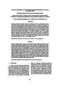
Then we have the monstrous curves: in 1890, Giuseppe Peano defined one, a line that fills a square and therefore can be considered two-dimensional. A few years later, in 1904, Helge von Koch devised another, reminiscent of a snowflake (see figure 1). This closed curve does not fill the plane, but has another anomalous property: its length seems to increase indefinitely as we look at it in more detail. In 1919, the mathematician H.Hausdorff proposed a new definition of dimension, to be applied in these dubious cases, to distinguish them from typical lines and surfaces. According to his definition, further refined by A.S. Besicovitch, monstrous curves may have a fractional dimension that to some extent measures the ratio between how much the curve grows in length and how much it advances. Thus, von Koch's snowflake curve has a Hausdorff-Besicovitch dimension equal to log 4 ----- = 1,2618595071429... log 3

On the other hand, Peano's curve has a Hausdorff-Besicovitch dimension of 2, and thus is analogous to a surface. Other definitions of fractals and fractal dimensions can be found in the literature [2, 3]. There are three main classes of fractal curves. Some appear as the boundary between the convergence and divergence of certain mathematical functions; others are generated by means of random Brownian movements; a third class includes those curves obtained when a recursive transformation is applied to an initial shape. Peano and von Koch monstrous curves are both in the latter group.

3

Representation of ASN.1 in APL nested structures

Lindenmayer Grammars The well-known Chomsky grammars have been used in theoretical computer science and language theory since the 1950s. In 1968, Aristid Lindenmayer [4] defined a new class of grammars (parallel derivation grammars), also called Lindenmayer systems or grammars or, in short, L systems. They are similar to Chomsky grammars, with an important difference: in the latter, a word generates another at each step of derivation by applying a rule that transforms a single symbol in the word into another string. In L systems, however, a word generates another by applying several rules simultaneously (one per every symbol in the word). Let us look at an example of an L system: if we have the rules A ::= B B ::= AB

and start at the word A, we get the following successive derivations: A → B → AB → BAB → ABBAB → BABABBAB ...

The lengths of the words in this series are 1,1,2,3,5,8,13,21,..., i.e. the Fibonacci series. There are different kinds of L systems, such as the following: • IL systems, context sensitive. • 0L systems, context free. • EL systems, with extensions. • TL systems, with tables. • DL systems, deterministic. • PL systems, propagative.

Different kinds of L systems may be combined: D0L systems are deterministic context free; PD0L systems are propagative deterministic context free; EIL systems are context sensitive with extensions; and so forth. L systems have been applied successfully to simulate different biological processes, such as the growth of plants, the shape of their leaves, their distribution around a twig, the pigmentation of snail shells, the growth of antlers... They have also been applied to represent complex systems such as fractal curves and cellular automata.

Fractal Representation by means of Lindenmayer Grammars Lindenmayer grammars provide a powerful tool to represent fractals of the recursive transformation type, such as Peano and von Koch monstrous curves. The recursive transformation may be easily represented by means of a grammar rule, and the initial shape by means of the initial word (the axiom of the L system). The fractal curve can be obtained from the series of words derived from the axiom by applying a certain graphic representation scheme. One of two main schemes are usually applied: vector graphics (which associates a fixed vector displacement to every symbol in the L system alphabet), or turtle graphics, where the letters are considered as the movements in the graphic space of a turtle that remembers its position and


4

preceding direction. We have proved [5] that both schemes are equivalent for an interesting set of fractal curves. As an example, let us consider the PD0L system defined by the axiom F+F--F+F and the following set of rules: F ::= F+F--F+F + ::= + - ::= -

The first derivation obtained from the axiom is: F+F--F+F → F+F--F+F+F+F--F+F--F+F--F+F+F+F--F+F

We obtain successive approximations to von Koch's snowflake curve if we apply to the derivations of this system the following turtle graphics interpretation: • F moves the turtle one step forward in its current direction. • + increases by 60 degrees the current angle of the turtle direction. • - decreases by 60 degrees the current angle of the turtle direction.

Figure 1 shows the graphical representation of the fifth derivation in the preceding L system. APL and J have been used before to process and display fractal curves [6]. In a previous paper [7] we have described our own approach, based on the representation of fractals by means of Lindenmayer grammars. We have developed an APL2 program that makes it easy to build Lindenmayer grammars and provides operations such as derivation and drawing according to either of the two above-mentioned graphic representation schemes.

Computation of the Fractal Dimension from the L System We have tackled the problem of determining the dimension of a fractal from its representation as a grammar. The first thing we had to do was to choose an appropriate definition for the fractal dimension. As mentioned above, different extensions to the concept of dimension have been proposed during the twentieth century, such as the Hausdorff dimension, the HausdorffBesicovitch dimension, the Minkowsky dimension and the box-counting dimension. Different techniques have been used to measure the fractal dimension as a ratio between how much the curve grows in length and how much it advances. We have tried to derive a fractal dimension by operating directly on the L system that represents the fractal curve by means of a turtle graphics representation. As explained, each word in the derivation represents a given configuration of the recursive generation of the fractal curve. The production rules embody the allowed transformation between configurations. Therefore, the growth of the words is related to the corresponding growth of the curve. The graphic interpretation of the L system makes it possible to assign bi-dimensional co-ordinates to the letters in each word. Once these co-ordinates have been computed, it is easy to obtain the distances between different points, which can be used as a measure of how much the curve grows in length. Performing operations on strings is an easier method of obtaining a fractal dimension than the computation of a limit.

5


Informally, our algorithm takes advantage of the fact that the right sides of the rules in the grammar provide a symbolic description of the fractal generator. We compute two numbers: the length N of the visible walk followed by the fractal generator in subsequent derivations, and the distance d in a straight line from the start to the end point of the walk, measured in turtle step units (this number can also be deduced from the rule string). The fractal dimension would then be: log(N) D = -----log(d)

The length N of the visible walk is not always equal to the number of symbols to be drawn in the generator string. This may happen because the turtle graphic associated with the rule strings or their derivations passes more than once along a set of points with a non-zero measure. Our algorithm has been refined to take this case into account in such a way that, in the computation of N, such sets of points are counted only once. This means that the value of N may be non-integer.

APL2 Implementation of the Algorithm We have developed a set of APL2 functions that compute the two numbers N and d, and calculate the box-counting fractal dimension with the preceding formula. We describe a fractal represented by an L system by a three or four component general vector containing: • The rules of the L system • Its graphic representation class (turtle or vector graphics) • Additional information related to the graphics representation • Optional comments

In the case of turtle graphics (the only we use here) the additional information in the third element is a two-element general vector containing the incremental angle, and the optional sets of invisible-move and non-graphic symbols. This representation of fractal curves is the same we used in our previous work, described in [7]. The main function in our APL2 implementation of the algorithm is called LDIMEN and receives as its only argument a three-element general vector containing: • The fractal (as described above) • The axiom (the starting string) • The number of iterations to be computed The function LDIMEN has the following code:

>@./',0(1;58/(61,1'(;$/)$&/$66$$1*/(7B3$,17


6

>@Æ&RPSXWHVIUDFWDOGLPHQVLRQIURPDQ/V\VWHPUHSUHVHQWDWLRQ >@58/(6;1 ;Æ/6\VWHP$[LRP1XPEHURILWHUDWLRQV >@58/(6&/$66$1*/( ¨58/(6Æ5XOHV&ODVV*UDSKLFLQIR >@ ±È$1*/( $1*/(7B3$,17 $1*/( Æ$QJOH6\PEVHWV >@$/)$58/(6>@Æ([WUDFWV\PERODOSKDEHWIURPWKHUXOHV >@.È; >@,1'(; >@/31È. >@;58/(6'/; >@$7857/(; >@..5(&2$ Ø',67$ >@/3 Lines 2-5 separate all the components of the argument X into appropriate variables. Lines 8 to 12 make the derivation loop. Auxiliary function D0L (reused at line 9 from our previous work) applies to string X one step of derivation by the L system defined by variable RULES. X, initialized to the axiom in line [2], is replaced by the new derivation. Function TURTLE2 applies the turtle graphics scheme to X and computes the set of points of the turtle trajectory. Functions RECO and DIST compute the values of N and d from that set of points, from which the estimated fractal dimension is obtained and kept in variable K, the result of the function. The actual fractal dimension is the limit of the series in K when the number of derivations tends to infinity. However, in many cases a single computation of the loop is enough to get the appropriate dimension, since all the terms in the series are the same. The set of points in the turtle trajectory do not cover the plane, since they must all be accessible from the starting point through a finite number of unitary vectors with angles multiples of the elementary turtle angle, which we limit to a value of 2kπ/n, with integer k and n. Most fractals in the literature agree with this limitation, which does not significantly restrict the usefulness of our approach. A Cartesian X-Y representation is not appropriate to define the points in the turtle trajectories, for their co-ordinates would be irrational in most cases, which means that they cannot be represented exactly in a computer. With APL2, the maximum precision of the mantissa of real numbers is 52 bits, and the errors would accumulate with the turtle movements, growing rapidly to unacceptable amounts. Remember that a turtle trajectory may consist of thousands of points, and the co-ordinates of each depend on the co-ordinates of all the previous points in the trajectory. An arbitrary precision representation of real numbers (using integers or character strings) is not the answer, since irrational numbers would have infinite many digits and would not be representable in any case. The fact that vector addition is commutative, and the number of different vectors that may be used to generate a turtle trajectory is finite, means that the position of a point reachable by the turtle from the origin may be expressed by a set of n non-negative integers, which indicate how many of the n possible unit vectors have been used to arrive there (see figure 2). This gives us the possibility to represent the exact position of every point using only a set of integer numbers: (0,1,1,1,2,1,2,1) for the point shown in figure 2. To make the representation unique for every point, we need to make sure that the walk of the turtle from the origin to the point is minimal. This means that we must eliminate all the loops in the trajectory which are regular polygons with a number of sides a submultiple of n (in actual fact, just the prime divisors of n have to be considered). If n is even, there is an additional situation: the fact that a section of a loop, larger than half a polygon, may be replaced by a smaller walk that goes around the remainder of the polygon in the opposite direction (see figure

7


3). We have written the following APL2 function that performs these changes and converts the representation of a point in the turtle trajectory into its minimal canonical representation:

>@=&$121;1,-)$ >@))Ö )35,0(B)$&1È=; >@ _1 // >@/== =Æ&DQRQLFIRUPIRUWKHFDVHRIRGG1 >@ È) >@=$1Ø$¨) È= >@==> ,2@ Ò= >@==º)©)º/ >@/==>@ Ò=1Ø È=Æ&DQRQLFIRUPIRUWKHFDVHRIHYHQ1 >@ È) >@=×$ 1Ø×$¨) È= >@, >@/-Ä$È AÕà$¨àÎß×$ ÊàÄ=>,@ Î >@-!×$ / >@=>-,@=>-×$ _ß-Î$,@$Èßº/ >@/1Ø×$ Ô,, / >@==º)©)º/ The function consists of two loops, one around label L1 (which takes care of odd n) and the other around label L2 (for cases of even n). Figure 4 shows an example of the use of this function to compute the canonical representation of a point in a fractal with an angle increment of 60 degrees. Function CANON is invoked by function TURTLE2 to make sure that every point in the turtle trajectory is represented by its canonical representation. Function DIST, that computes the value of d (the straight distance between the starting and the end points in the string that represents one of the steps driving to the fractal curve), is trivial:

>@=',67$ >@=&$57(6©$>¨È$@ &$57(6©$>@ where CARTES is a function that converts our canonical representation of a point into its Cartesian representation:

>@=&$57(6; >@=;×>@ÚÌÌÎßÈ; ×9(&725Ø Function RECO, that computes the value of N (the length of the visible walk) is more complicated, as it must eliminate all repetitions. This is the least efficient function in our algorithm. However, if we know that there are no repetitions in the turtle walk, this function can be replaced by a much more efficient version. The most general version of this function is:

>@=5(&2$,-333334 >@= >@/aÐ$>@ >@,$>@Î >@3©$>,@ >@3©$>,@Æ33HQGVRIQH[WVHJPHQW >@- >@/-Ô, / >@$>-@ / >@3©$>-@ >@3©$>-@Æ33DOUHDG\UHYLVHGVHJPHQWV >@a_33 ±_33 / >@3±3 A3±3 Í3±3 A3±3 /


8

>@33(175(33 >@43(175(33 >@3A4 / >@a3Í4 / >@ 4 33 33 >@33(175(33 >@3/$ >@33º/ >@/$33 >@//-- >@/==&$57(63 &$57(63 >@//$>,@ß where function ENTRE returns 1 if the point at its left argument is located in the segment connecting the two points at its right argument and 0 otherwise.

Examples of Use In the next, we show a few additional examples of fractals typical in the literature. We have used function LDIMEN to compute their fractal dimensions. In all cases, the results we have obtained agree with those arrived at by other, mainly graphical, methods. The PD0L scheme F ::= +F--F++F+::=+ -::=-

with axiom F++F++F++F++F++F, and a turtle graphic interpretation, where F is a draw symbol, and the step angle is 30 degrees, represents the fractal whose first four derivations appear in figure 5. The values of N and d , obtained with our functions, are 3 and the square root of 7. Therefore, the dimension is: D=

log(9) = log(7)

1,12915...

in accord with Mandelbrot's results in reference [1], page 46.

The PD0L scheme F ::= F+F-F-FF+F+F-F +::=+ -::=-

with axiom F-F-F-F, and a turtle graphic interpretation, where F is a draw symbol, and the step angle is 90 degrees, represents the fractal whose first three derivations appear in figure 6. In this case, N and d are computed to be 8 and 4. Therefore, the dimension is: D=

log(8) = log(4)

= 1,5

9



The PD0L scheme F ::= +F-F+F+F-F-FF+F-F-FF-F+F+FF-FF+FF-F-F+FF+F+F-FF+F+F-F-F+F+::=+ -::=-

with axiom F-F-F-F, and a turtle graphic interpretation, where F is a draw symbol, and the step angle is 90 degrees, represents the fractal whose first two derivations appear in figure 7. The values of N and d, obtained from this L system, are 32 and 8. Therefore, the dimension is: D=

log(32) = log(8)

1,6666...


Conclusions APL has been shown to be a powerful language for the representation of fractal curves. In the research described in this paper (we have used IBM’s APL2), we have developed a new algorithm that provides a novel way to compute the fractal dimension of a curve by means of symbol manipulation, without using graphical procedures. The fact that APL2 is a very good language for the manipulation of symbols and complex data structures, makes it very appropriate for this kind of applications.

References [1] Mandelbrot, B.B.: The Fractal Geometry of Nature, W.H.Freeman and Company, New York, 1977. [2] Falconer, K.: Fractal Geometry: Mathematical Foundations and Applications, John Wiley & Sons, Chichester, 1990. [3] Masaya Yamaguti, Masayoshi Hata, Jun Kigami. Mathematics of fractals, Translation of Mathematical Monographs, volume 167. American Mathematical Society, Providence, 1993. [4] Lindenmayer, A.: Mathematical models for cellular interactions in development (two parts). J. Theor. Biol. 18, pp. 280-315, 1968. [5] Alfonseca, M.; Ortega, A.: A study of the representation of fractal curves by L systems and their equivalences. IBM Journal of Research and Development, Vol. 41:6, p.727-736, Nov. 1997. [6] Reiter, C.A.: Fractals RYIJ, Vector, Vol. 11:2, p. 86-104, Oct. 1994. [7] Alfonseca, M.; Ortega, A.: Representation of Fractal Curves by means of L Systems, APL Quote Quad (ACM SIGAPL), Vol. 26:4, p. 13-21, Jun. 1996. Presented at APL 96, Lancaster, Jul. 1996.


Figure 1

Figure 2

10

11

Figure 3



Figure 4

12

13

Figure 5



Figure 6

14

15

Figure 7
