Using Background Knowledge to Build Multistrategy Learners
Claude Sammut School of Computer Science and Engineering University of New South Wales Sydney Australia 2052
[email protected]
Abstract This paper discusses the role that background knowledge can play in building flexible multistrategy learning systems. We contend that a variety of learning strategies can be embodied in the background knowledge provided to a general purpose learning algorithm. To be effective, the general purpose algorithm must have a mechanism for learning new concept descriptions that can refer to knowledge provided by the user or learned during some other task. The method of knowledge representation is a central problem in designing such a system since it should be possible to specify background knowledge in such a way that the learner can apply its knowledge to new information.
1. Introduction There are many reasons why one may wish to combine a variety of learning strategies in one system. Many experiments have confirmed that we are yet to find a single learning algorithm that does best in all circumstances (for example, Michie, Spiegelhalter & Taylor, 1994). It is often more effective to use different algorithms at different times than to try to use one algorithm all the time. This approach raises several questions, including: under which circumstances is a particular method appropriate and how large does our library of algorithms have to be? Often, multistrategy learning systems have a fixed set of algorithms to draw upon and their interaction is pre-determined by the programmer. In other words, they are often designed to be specific to a particular type of learning problem. In this paper, we suggest that general purpose multistrategy learners can be constructed by allowing the learner to make use of complex background knowledge.
1
Human Trainer
As the trainer flies the aircraft, all of his/her actions are recorded
Flight Log
Flight Simulator
Learning Program
Auto-pilot
An induction program
The rules are put into an
uses the flight log to
autopilot which can fly
build rules for flying
the simulated aircraft
Figure 1. Learning to Fly We contend that a great deal of flexibility can be gained by a machine learning system that uses a concept representation language that permits references to user defined background knowledge as well as knowledge derived from other learning tasks. First, we illustrate the power of complex background knowledge with an example of numerical reasoning in inductive logic programming. Next, we describe a machine learning system that encourages the use of learned as well as predefined background knowledge. Finally, we discuss the connection between background knowledge and multistrategy learning.
2. An Example: Numerical Reasoning in ILP The effectiveness of background knowledge as a means of providing a variety of learning strategies can best be seen through an example. Sammut, Hurst, Kedzier and Michie (1992) describe a learning problem where a human pilot is required to fly an aircraft in a flight simulator. During the flight the actions of the pilot are logged, along with the situation in which the action is performed. Flight logs are used as input to an induction program which generates rules for an autopilot. The architecture of the system is illustrated in Figure 1. The task of piloting an aircraft through a complete flight plan is a complex task involving a number of stages, each of which is defined by a particular goal. For
Take off and climb to 2000 feet Fly straight and level Turn to heading 330˚
Land Approach runway
Turn
Line up
Figure 2. Stages of a flight. example, the pilot may be told to take off; climb to a particular altitude; turn to some heading; maintain straight and level flight until a certain marker is reached, etc. An example of a multi-stage flight is shown in Figure 2. For each stage of a flight, we build a separate set of control rules. Further complexity is added by the fact that an aircraft has a number of controls, eg. elevators, ailerons, rudder, flaps, throttle, etc. Within each stage we build rules for each control available to the pilot. The result is a two-level controller where the top level is an “executive” which invokes low level agents to perform a particular task. Thus, “Learning to Fly” applies machine learning in a number of ways to build a control system that has different strategies for different situations. While the result is a multistrategy controller, our original experiments only involved a single learning algorithm, C4.5 (Quinlan, 1993). Although these experiments resulted in working autopilots capable of flying the aircraft from take-off to landing, the rules that were generated were often large, difficult to read and not always robust under different flight conditions. One reason for some of these difficulties is that only the raw data from the simulator were presented to the learning algorithm. The data obtained from the simulator include the position, orientation and velocities of the aircraft as well as the control settings. While these data are complete in the sense that they contain all the information necessary to describe the state of the system, they are not necessarily presented in the most convenient form. For example when a pilot is executing a constant rate turn, it makes sense to talk about trajectories as arcs of a circle. Induction algorithms, such as C4.5, can deal with numeric attributes to the extent that they can introduce in
3
equalities, but they are not able to recognise trajectories as arcs or recognise any other kind of mathematical property of the data. Srinivasan and Camacho (forthcoming) have shown how such trajectories can be recognised with the aid of a sophisticated mechanism for making use of background knowledge. This mechanism is part of the inductive logic programming system Progol (Muggleton, 1995). The feature of Progol that most interests us here is that the learning algorithm is embedded in a custom built Prolog interpreter. Concepts learned by Progol are expressed in the form of Prolog Horn clauses and background knowledge is also expressed in the same form. Moreover, the Prolog interpreter’s built-in predicates may appear in either learned or background clauses. 2.1 Background Knowledge and Generalisation Like Marvin (Sammut, 1981; Sammut & Banerji, 1986), Progol begins by taking the description of a single positive example and saturates the description by adding to it literals derived from background knowledge. The new literals result from background predicates being satisfied by data in the example. To illustrate this, let us consider Michalski’s (1983) categorisation a number of generalisation operations. For example, “climbing a generalisation tree” is one type of generalisation operation. Let us define a simple type hierarchy in terms of Horn clauses. living_thing(X) :- plant(X). living_thing(X) :- animal(X). animal(X) :- mammal(X). animal(X) :- fish(X). mammal(X) :- elephant(X). mammal(X) :- whale(X).
Suppose ‘fred’ is an example of the concept ‘p’ which we wish to learn. Fred has the property that it is an elephant. p(fred) :- elephant(fred).
Saturation (Rouveirol, 1990) proceeds as follows: mammal(fred) is true since elephant(fred) is given. Having concluded mammal(fred), animal(fred) follows and consequently so does living_thing(fred). A system like Progol would construct a most specific clause like: p(fred) :elephant(fred), mammal(fred), animal(fred), living_thing(fred).
p(X).
p(X) :- ....
p(fred) :- elephant(fred), mammal(fred), animal(fred), living_thing(fred).
Figure 3. Generalisation lattice This forms the most specific clause at the bottom of a generalisation lattice. An example of such a lattice is shown in Figure 3. The most general clause is the clause with no body. Each node in the lattice is a clause whose body is a subset of the literals in the body of the most specific clause. The learning algorithm must search this lattice for the clause the best describes the positive examples while excluding the negative examples. Note that the lattice is very similar to Mitchell’s version space (Mitchell, 1977) When saturation is completed, Progol uses the most specific clause to serve as a bound on a general-to-specific search. Beginning with the most general clause, ie. one with an empty body, Progol tries to find a subset of the most specific clause that satisfies a minimum description length criterion for the best clause. Muggleton (1995) describes the search procedure. Suppose the background knowledge contains the clauses: X in L..H :- X >= L, L =< H.
and the example, p(2, 1, 3).
is presented to the learning system, then a generalisation is: p(N, X, Y) :- N in X..Y.
since 2 in 1..3 is satisfied. Thus, Michalski’s “closing the interval” rule can also be obtained from background knowledge. Like many ILP systems (De Raedt, 1996), Progol permits mode declarations which provide a declarative bias to restrict the
5
Table 1. Background Predicates pos(P, T)
position, P, of aircraft at time, T.
before(T1, T2)
time, T1, is before time, T2.
regression(ListY, ListX, M, C)
least-square linear regression, which tries to find Y = M × X + C for the list of X and Y values.
linear(X, Y, M, C)
linear(X, Y, M, C) :- Y is M*X+C.
circle(P1, P2, P3, X, Y, R)
fits a circle to three points, specifying the centre (X, Y) and radius, R
==, abs
Prolog built-in predicates
application of predicates to avoid an explosion in the number of literals that the saturation procedure may construct. Note that in the example above, we used one of Prolog’s built-in arithmetic predicates “= Lens = none |TearProduction = normal -> (Astigmatism = not_astigmatic -> Lens = soft |Astigmatism = astigmatic -> (Prescription = myope -> Lens = hard |Prescription = hypermetrope -> |Age = pre_presbyopic -> Lens = none |Age = presbyopic -> Lens = none)))).
Learning programs that follow similar paradigms use the same notation. So, for example, if the user wished to compare decision trees versus Gaines’ Induct-RDR (Gaines, 1989), it would only be necessary to invoke another command: induct(lens)?
Which results in the rule:
3
Although iProlog generally follows the ISO Prolog standard, there are some minor differences. The postfix ‘?’ operator is used in preference to the standard prefix ‘?-’ to invoke the prolog interpreter. The ‘|’ in if-thenelse constructs is a synonym for the ‘;’ (th or operator). 9
lens(Age, Prescription, Astigmatism, Tear_production, Lens) :(Lens = none unless (Astigmatism=not_astigmatic, Tear_production=normal -> Lens=soft unless (Age = presbyopic, Prescription = myope -> Lens = none) |Prescription = myope, Tear_production = normal -> Lens = hard |Age = young, Tear_production = normal -> Lens = hard)).
Induct-RDR uses Compton’s Ripple-down Rule representation (Compton & Jansen, 1988). An unless operator has been added to Prolog’s standard if-then-else construct. The example above is read as “lens is none unless not astigmatic and tear production is normal. In that case the conclusion is that the lens should be soft. This conclusion is over-ridden if age is presbyopic, ...” So far, an Aq algorithm (Michalski, 1973; 1986) and a naive Bayes classifier also follow the same notation. 3.2 Numerical Algorithms and Filters The training instances shown so far have been stored as ground unit clauses in Prolog’s database. That is, the relation is represented by the examples in extensional form. One of the useful features of storing examples as Prolog clauses is that, in execution, there is no difference to the caller whether the relation is implemented extensionally or intentionally. Thus, examples maybe generated by a Prolog program. We use the task of learning to fly again to show how this feature can be used. Suppose the data logged from the simulator are described by the following mode declaration: mode flight1(+x, +y, +z, +x_vel, +y_vel, +z_vel, +roll, +pitch, +heading, +roll_rate, +pitch_rate, +yaw_rate, –elevators, +ailerons, +rudder, +flaps, +speed_break, +lg1, +lg2, +lg3, +throttle, +rpm).
These data are all numeric and we will use a learning algorithm that produces numeric output, like CART’s regression trees (Breiman et al, 1984). The variables represent the position, orientation and velocities of the aircraft as well as the current control settings. For numeric problems, we use a notation based on DEC-10 Prolog’s mode declarations. The independent variables are marked with a “+” and the dependent variable is marked with a “–”. In this case we wish to predict the elevator setting given the other variables as input. Like the decision tree program, a regression tree algorithm is simply invoked by passing the relation name as the argument to a procedure call: rt(flght1)?
The raw data provided are often not in a form most suitable for analysis. For example, rather than have separate x, y and z velocities as given above, we may prefer to use the single value of airspeed. We may also decide that some variables,
such as the position of the landing gear (lg1, lg2 and lg3) are not relevant. We can define a new relation derived from the old one as follows: mode flight2(+airspeed, +climb_rate, +roll, +pitch, +heading, +roll_rate, +pitch_rate, +yaw_rate, –elevators, +ailerons, +rudder, +flaps, +speed_break, +throttle,+rpm). flight2(AirSpeed,ClimbRate,Roll,Pitch,Heading,RollRate,PitchRate,YawRate,Elevators,Ailerons,Rudder,Flaps, SpeedBreak,Throttle,RPM) :– flight(X,Y,Z,Xvel,Yvel,Zvel,Roll,Pitch,Heading,RollRate,PitchRate,YawRate,Elevators,Ailerons,Rudder, Flaps,SpeedBreak,0,0,0,Throttle,RPM), AirSpeed is sqrt(Xvel*Xvel + Yvel*Yvel + Zvel*Zvel), ClimbRate = Zvel.
To build a new regression tree now, we call: rt(flght2)?
Induction algorithm usually read their data from files. Instead, a learning algorithm in iProlog invokes the Prolog interpreter to deliver its examples. When examples are stored extensionally, this is just the same as reading one example at a time. However, in the case above, we have redefined the relation. If we ask for all solutions of the relation flight2, we get the original data filtered by a program that calculates the airspeed and only delivers those examples where the landing gear is up (0 for all three wheels). Although this kind of filtering can be done by preprocessing input files to any learning program, the ease with which data can be transformed in this environment saves a great deal of time. We will also see later that filters are important in multistrategy learning. Like the classification programs, the output from a regression tree algorithm is also a valid Prolog program. For example, the following data are extracted from a larger data set: pitch(500, pitch(498, pitch(489, pitch(413, pitch(397, pitch(369, pitch(265, pitch(252, pitch(231, pitch(211, pitch(202, pitch(195,
-2461, -2422, -2385, -2219, -2190, -2131, -1925, -1895, -1835, -1771, -1737, -1702,
-977, -955, -932, -801, -771, -709, -494, -463, -400, -339, -311, -283,
-7). -17). -20). -20). -18). -19). -15). -13). -12). -10). -8). -7).
Running the regression tree program on these data, we obtain:
11
pitch(Alt, Dist, X, Pitch) :(Alt (Alt Pitch = -3.86; (Alt Pitch = -7.70; Pitch = -6.11)); Pitch = -17.18).
Statistical techniques such as a linear discriminant algorithm (Fisher, 1936)4 and connectionist methods like back-propagation (Werbos, 1975; Hinton, Rumelhart & Williams, 1985) can also be used to create numerical relationships. To illustrate how a back-propagation network can be integrated into an ILP setting, let us see how the classic xor network can be represented. The original xor relation is: xor(0, xor(1, xor(1, xor(0,
0, 0, 1, 1,
0). 1). 0). 1).
A network with two hidden nodes is trained on the above data and the resulting network is described by the clause: xor(Input1, Input2, Output) :X10 is logistic(3.01981 + -6.05867 * Input1 + 6.32054 * Input2), X11 is logistic(-3.6811 + -6.7386 * Input1 + 6.76381 * Input2), Output is logistic(4.91949 + -10.2493 * X10 + 10.4417 * X11).
The function, logistic , is required to provide the standard activation function, 1 1 + e− x Thus, we have a new classifier which can be invoked as a Prolog program and, like any other program, can be used as background knowledge.
4. Structured Induction and Exploratory Data Analysis The present solution to the “Learning to Fly” task is an example of structured induction. Shapiro (1987) introduced the idea of structured induction as a means of simplifying a learning task and for making the result of learning more human readable. His experiments were conducted in the familiar domain of chess endgames. Quinlan (1979) had previously demonstrated that it was possible to induce decision trees for this domain. However, they were usually large and end-game experts could find little in them that corresponded to their own intuition. To
4Adapted
from Bob Henery’s Statlog code (Michie, Spiegel,halter & Taylor, 1994)
overcome this problem, Shapiro obtained the help of a chess master who was able to describe high-level features that players looked for. Armed with this knowledge, Shapiro induced decision trees for each of the highlevel features and organised the whole knowledge base as a tree of trees. The toplevel tree was hand-crafted from the knowledge obtained by the chess expert. The subtrees were built by induction. The result was an accurate solution which also made sense to chess experts. Shapiro used a uniform representation and the same type of induction algorithm throughout his analysis. This is also true of the original flight control system. All the control agents were synthesised using the same learning algorithm. However, in the iProlog framework, different algorithms may be used when one is more appropriate than another. Since they all generate Prolog programs, the task of invoking the ‘lowlevel’ knowledge from the ‘high-level’ can be done simply by constructing clauses for the high-level knowledge which calls the induced procedures. Used in this manner, our multistrategy learning is not fully automatic, but rather, is a collaboration between human and machine. In practical data analysis, it is most likely that the human user will want quite a lot of discretion in choosing strategies and guiding induction. Therefore, we do not force too much automation on the user, but prefer to provide building blocks. To be a useful tool, particularly for applications in data mining, the machine learning environment must provide for “what if” experiments in which the user may try something, then try something else, come back to a previous experiment, etc. Logically, when a new rule is induced it could replace the ground facts that were used as examples during induction. That is, a new, more general, theory replaces the older theory. However, its unlikely that a user would wish the original data to be destroyed as this would prevent further experimentation, unless the data were completely reloaded. One approach to permitting ‘what-if’ experiments is to create a separate database for induced rules. For example, when the decision tree algorithm os run on the lens data, the system builds a ‘frame’ containing the following information:
13
creator: id(lens); date: '97/08/22 - 12:55:12'; n_examples: 24; errors: 0; time: 0.0166667; rule: lens(Age, Prescription, Astigmatism, Tear_production, Lens) :(Tear_production = reduced -> Lens = none |Tear_production = normal -> (Astigmatism = not_astigmatic -> Lens = soft |Astigmatism = astigmatic -> (Prescription = myope -> Lens = hard |Prescription = hypermetrope -> (Age = young -> Lens = hard |Age = pre_presbyopic -> Lens = none |Age = presbyopic -> Lens = none)))).
As well as building the rule for the concept, the system stores the procedure call that created the rule. This is useful because, the programs may have parameters such as pruning levels or learning rates, and these will be recorded. Other information such as the number of examples, number of errors on training and test data, etc can also be stored. Thus comparisons of different learning trails are easy to do . Thus the user is aided in making an appropriate choice of algorithms, parameters, attributes, etc.
5. Multistrategy Learning So far, we have seen how a variety of learning algorithms can be incorporated into a single framework to provide a convenient environment for data exploration. But more than being just a another machine learning tool kit, that fact that all the algorithms use a common language means that it is easy to pass the results of one algorithm to another. Therefore one learning algorithm can make use of another. In section 2.2 we saw how Srinivasan used Progol to mix data fitting strategies. Let us see how this approach can be generalised. The first point to note is the system will probably need some guidance, in the form of a language bias. Because first order representation languages are so rich, the search space for a learning algorithm can be prohibitively large unless, the search space is restricted in some way. Many first order learning systems allow the user to write ‘mode declarations’ or define a refinement operator which restrict the concept description language to a tractable subset of Horn clause logic. Thus the user must have at least some rough ideas about what the learning system should look for. In that sense, data analysis is a cooperative endeavour between human and computer. The language bias tells the learning algorithm which background predicates to add during saturation. Normally, background predicates are complete at the time of
learning. For example, our animal taxonomy in section 2.1 would have been entered before starting any learning task involving animals. This was not the case for learning the relationship between roll angle and turning radius. Linear regression was used to generate a background predicate ‘on-the-fly’. To do this, two mod declarations were need. One was used during learning to instruct Progol to try linear regression and a second mode declaration was used to actually construct the literal that implemented linear equation in the concept description. Furthermore, the ‘learning time’ mode declaration had to indicate that all the values of a variable had to be collected in order to perform the regression. Because of its flexibility, we have chosen a method of language bias based on Cohen’s refinement rules (Cohen, 1996). Cohen gives an example of refinement rules that may be used in the king-rook-king illegal problem: DB0 = {rel(adjacent), rel(equal), rel(less_than)} illegal(A, B, C, D, E, F) ← where true asserting {row(A), col(B), ..., row(E), col(F)} ← R(X, Y) where rel(R), CommonType(X), CommonType(Y) asserting ∅ DB0 is an initial database which contains information that the refinement operation can use. In this case, the database starts with a list of the relations that refinement is allowed to use in building a clause. There are two types of refinement rules. There must be one and only one rule of the form ClauseHead ←. This tells the system what the head of the clause being learned should look like. Expressions of the form, where asserting inform the system about the conditions that must be true before the rule can be applied and the conditions which must apply afterward. The post conditions are added to DB. In this example, the first refinement rule indicates that the head of the clause should be illegal(A, B, C, D, E, F) and the arguments are rows or columns. Rules of the form, ← BodyLiteral, tell the system the form of literals that may be added to the body of the clause being learned. In this example, the rule indicates that literals like adjacent(X, Y), equal(X, Y) and less_than(X, Y) are legal as long as X and Y are of the same type. Refinement rules use a second order, language permitting predicate symbols to be variables. This notation is very convenient for multistrategy learning since literals in the precondition of a refinement rule can be calls to another learning algorithm. For example, we may have a data set that contains continuous attributes and we wish to 15
try a regression tree algorithm on some of those attributes. In the flight data, one option we want the program to explore is a relationship between the pitch angle and the location of the aircraft5. The following refinement rule accomplishes that. ← pitch(Alt, Dist, X, Pitch) where rt(pitch) asserting ∅ When the pre-condition for adding the pitch literal is checked, the regression tree program is invoked, generating the clause shown in section 4.2. The pitch literal is then a reference to this newly generated clause. If the pitch data are not stored explicitly, as in our earlier example, it may be necessary to have a filter program, similar to flight2, to define the pitch relation based on the four variables above in the full flight data. Of course, the learning systems search algorithm must still determine whether a literal generated by this rule is useful. We now have a mechanism that allows the system to automatically explore a combination of different types of background knowledge, including other learning algorithms, based on suggestions provided by the user.
6. Propositional versus First order Learning One of the difficulties that advocates of first order learning face is finding a convincing argument why it is necessary. Common counter arguments are that problems that may naturally be represented in a first order form can often be transformed into propositional form and propositional learners (eg. decision trees, etc) are much faster than first order learners. Clearly there are some problems, such as learning programs like list membership, sorting, etc, for which it is not possible to make such a transformation. However, for many real-world problems, the counter argument is a powerful one. The main contention of this paper is that the primary advantage of first order representations is the ease with which background knowledge can be incorporated in the learning framework. However, this need not force the user to incur a penalty in efficiency. Lavraˇc and Dˇzeroski (1994) describe the LINUS algorithm in which problems are presented in a first order representation and then transformed into a propositional form for input to a learning program such as CN2 (Clark & Niblett, 1989; Clark & Boswell, 1991). Why do this? Why not start with a propositional representation? The most obvious answer is that some domains, like molecular biology (Muggleton, King 5
This is not really a very useful relation, but it serves our purpose as an example.
& Sternberg, 1992) and natural language processing (Mooney & Califf, 1995) are most naturally represented using first order theories. But the most compelling reason, ultimately, is that in the first-order form, it is easy to use a method like saturation to elaborate the description of the training examples based on background knowledge, prior to transformation. Turney (1996) used a similar transformational approach in response to Michie et al’s (1994) East-West Challenge. Here that task was to learn to classify East-bound and West-bound trains according to features such as types of carriages and their loads, etc. However, some relations were also required to successfully represent the trains. After transformation, Turney’s system generated training examples with 1199 features . The relational representation was for more compact and therefore more easily understood by humans, but the feature vector permitted a fast propositional learner to be applied. In the experiments reported previously, Srinivasan used linear regression as background knowledge for an ILP system. In subsequent work, (Srinivasan, 1996) he reversed the rôles of ILP and statistics. The task for his learning system this time, was, given the chemical structure of some molecules to obtain descriptions relating structure to activity. He noted the following: the domain is inherently quantitative and ILP is best suited to qualitative descriptions; when appropriate attributes have been available, ILP programs have not been able to better the performance of standard techniques like linear regression, however, ILP programs perform creditably when such attributes are unavailable; ILP programs are usually slower than their propositional counterparts. The attributes in this domain are usually supplied by experts. However, they are often unable to conceive a complete range of useful attributes. These observations lead Srinivasan to use ILP as a preprocessing stage for linear regression. He applied Progol to the data so that it could discover relations such as ‘compound has hydrogen at position 4 and the substituent at position 3 is a hydrogen donor’. Once discovered, these relations were turned into attributes to be used by a standard linear regression package. These experiments show that the title of this section is really misleading. There is no reason to think of propositional and first order learning systems to be in competition with each other. We have just discussed several examples where they have complemented each other. So, the question arises: is it possible to build a general framework within which various learning systems can be combined in a flexible way? We hope that this paper demonstrates that the answer to this question is “yes”, using logic programming to provide the framework.
17
7. Conclusion We have shown how a number of different learning algorithms can be incorporated into a unified environment for data exploration. Multistrategy learning can be accomplished by using one form of learning to construct background knowledge for another. The key features of the system that enable this kind of multistrategy learning are that: • the background knowledge and the concept description language are the same and • the concept descriptions generated by the learning programs are themselves executable as programs. A uniform representation language ensures that knowledge can be reused. That is, learned concepts can be added to background knowledge for further learning. The user can also provide pre-defined background knowledge and the system will not have to know what is user defined and what has been learned because both are treated the same way. Since the representation language is executable and can be used to write programs, the background knowledge can describe complex concepts, including other learning and data modelling algorithms. We have seen how a refinement language can be used to guide the system in selecting sub-tasks for learning. When a refinement operator seeks some background knowledge, it can invoke another learner to the background knowledge, on-the-fly. Examples of this kind of ‘sub-task’ learning were using regression to find numerical relationships for an ILP learner; using ILP to find attributes for regression and using regression trees to find numerical relations for an ILP learner. Because the definition of refinement operators is flexible, many different combinations of learning strategies are possible. The main reason for resorting to multistrategy learning is that different learning methods are better suited to different tasks. We have used Inductive Logic Programming as the framework in which a variety of learning systems can be embedded. The ILP framework was chosen because it allows very complex background knowledge to be encoded. Thus, while a particular learning algorithms can provide high performance for specific domains, ILP provides the ‘glue’ the binds the different learning strategies together.
Acknowledgments Thanks to Ashwin Srinivasan and Mike Bain for their assistance in understanding the intricacies of Progol.
References Bain, M., Sammut, C., Sharma, A., & Shepherd, J. (1996). ReDuce: Automatic structuring and compression in relational Databases. In MLnet Workshop on Data Mining with Inductive Logic Programming, (pp. 41-52). Bari, Italy. Breiman, L., Friedman, J. H., Olshen, R. A., & Stone, C. J. (1984). Classification and Regression Trees. Belmont, CA: Wadsworth International Group. Cendrowkska, J. (1987). An algorithm for Inducing Modular Rules. International Journal of Man-Machine Studies, 27(4): 349-370. Clark, P., & Boswell, R. (1991). Rule induction in CN2: Some recent improvements. In Proceedings of the Fifth European Working Session on Learning. (pp. 151-163). berlin: Springer. Clark, P., & Niblett, T. (1989). The CN2 induction algorithm. Machine Learning, 3(4), 261-283. Cohen, W. (1996). Learning to classify English text with ILP methods. In L. De Raedt (Eds.), Advances in Logic programming. (pp. 124-143). IOS Press. Compton, P. J., & Jansen, B. (1988). Knowledge in context: A strategy for expert system maintenance. In Proceedings of the Australian Artificial intelligence Conference, De Raedt, L. (Ed.). (1996). Advances in Logic Programming. IOS Press. Fisher, R. A. (1936). The use of multiple measurements in taxonomic problems. Annals of Eugenics, 7, 179-188. Gaines, B. R. (1989). An ounce of knowledge is worth a ton of data. In A. M. Segre (Ed.), Proceedings of the Sixth International Workshop on Machine Learning, 156-159. Ithaca, New York: Morgan Kaufmann. Hinton, G. E., Rumelhart, D. E. & Williams, R. J. (1985). Learning internal representation by back-propagating errors. In D. E. Rumelhart, J. L. McClelland & The PDP Research Group (Eds.), Parallel Distributed Computing: Explorations in the Microstructure of Cognition. (pp. 31-362). Cambridge, MA: MIT Press. Lavraˇc, N., & Dˇzeroski, S. (1994). Inductive Logic Programming: Techniques and Applications. Ellis Horwood.
19
Michalski, R. S. (1973). Discovering Classification Rules Using Variable Valued Logic System VL1. In Third International Joint Conference on Artificial Intelligence, 162172. Michalski, R. S. (1983). A Theory and Methodology of Inductive Learning. In R. S. Michalski, J. G. Carbonell, & T. M. Mitchell (Eds.), Machine Learning: An Artificial Intelligence Approach. Palo Alto: Tioga. Michalski, R. S., Mozetiˇc, I., Hong, J., & Lavraˇc, N. 1986. The multi-purpose incremental learning system AQ15 and its testing application to three medical domains. In Proceedings of AAAI-86, Philadelphia: Morgan Kaufmann. Michie, D., Muggleton, S., Page, D., & Srinivasan, A. (1994). To the international computing community: A new East-West challenge. Oxford University Computing Laboratory. (ftp://ftp.comlab.ox.ac.uk/pub/Packages/ILP/trains.tar.Z). Michie, D., Spiegelhalter, D. J., & Taylor, C. C. (Ed.). (1994). Machine Learning, Neural and Statistical Classification. Elis Horwood. Mitchell, T. M. (1977). Version Spaces: A Candidate Elimination Approach to RuleLearning. In Proceedings of the Fifth International Joint Conference on Artificial Intelligence, (pp. 305-310). Mooney, R. J., & Califf, M. E. (1995). Induction of first-order decision lists: Results on learning the past tense of English verbs. Journal of Artificial Intelligence Research, 2. Muggleton, S., King, R., & Sternberg, M. (1992). Predicting protein secondary structure using inductive logic programming. Protein Engineering, 5, 647-657. Muggleton, S. (1995). Mode-directed inverse resolution. New Generation Computing. Quinlan, J. R. (1979). Discovering rules by induction from large collections of examples. In D. Michie (Eds.), Expert Systems in the Micro-Electronic Age. Edinburgh: Edinburgh University Press. Quinlan, J. R. 1993. C4.5: Programs for Machine Learning. San Mateo, CA: Morgan Kaufmann. Rouveirol, C., & Puget, J.-F. (1990). Beyond Inversion of Resolution. In Proceedings of the Seventh International Conference on Machine Learning, Morgan Kaufmann. Sammut, C. A. (1981). Concept Learning by Experiment. In Seventh International Joint Conference on Artificial Intelligence. Vancouver. Sammut, C. A., & Banerji, R. B. (1986). Learning Concepts by Asking Questions. In R. S. Michalski Carbonell, J.G. and Mitchell, T.M. (Eds.), Machine Learning: An Artificial Intelligence Approach, Vol 2. 167-192. Los Altos, California: Morgan Kaufmann.
Sammut, C., Hurst, S., Kedzier, D., & Michie, D. (1992). Learning to Fly. In D. Sleeman & P. Edwards (Ed.), Proceedings of the Ninth International Conference on Machine Learning, Aberdeen: Morgan Kaufmann. Shapiro, A. (1987). Structured Induction in Expert Systems. Addison-Wesley. Srinivasan, A. (1996). Feature construction with Inductive Logic Programming: A study of quantitative predictions of chemical activity aided by structural attributes. In Proceedings of the Japanese Inductive Logic Programming Workshop, Saporro. Srinivasan, A & Camacho, R. (in press). Numerical Reasoning in ILP. In S. Muggleton, K. Furukawa & D. Michie (Ed.), Machine Intelligence 15. Oxford University Press. Turney, P. (1996). Low-size complexity inductive logic programming: the East-West Challenge as a problem in cost-sensitive classification. In L. De Raedt (Ed.), Advances in Logic Programming. (pp. 308-321). IOS Press. Werbos, P. (1975) Beyond Regression: New tools for prediction and analysis in the behavioural sciences. Ph.D. thesis, Harvard University.
21