Worst-Case Background Knowledge in Privacy - CiteSeerX

Worst-Case Background Knowledge in Privacy David Martin

Daniel Kifer

Ashwin Machanavajjhala Johannes Gehrke Joseph Halpern Cornell University {djm, dkifer, mvnak, johannes, halpern}@cs.cornell.edu

Abstract Recent work has shown the necessity of considering an attacker’s background knowledge when reasoning about privacy in data publishing. However, in practice, the data publisher does not know what background knowledge the attacker possesses. Thus, it is important to consider the worst-case. In this paper, we initiate a formal study of worst-case background knowledge. We propose a language that can express any background knowledge about the data. We provide a polynomial time algorithm to measure the amount of disclosure of sensitive information in the worst case, given that the attacker has at most k pieces of information in this language. We also provide a method to efficiently sanitize the data so that the amount of disclosure in the worst case is less than a specified threshold.

1. Introduction We consider the following situation. A data publisher (such as a hospital) has collected a useful information about a group of individuals (such as patient records that would help medical researchers) and would like to publish this data while preserving the privacy of the individuals involved. The information is stored as a table (as depicted in Figure 1), where each record corresponds to a unique individual and contains a sensitive attribute (e.g., disease) and some non-sensitive attributes (e.g., address, gender, age) that might be learned using data available externally (e.g., phone books, birth records). The data publisher would like to limit the disclosure of the sensitive values of the individuals in order to defend against an attacker who possibly already knows some facts about the table. Our goal in this paper is to quantify the precise effect of background knowledge possessed by an attacker on the amount of disclosure and to provide algorithms to check and ensure that the amount of disclosure is less than a specified threshold. The problem we solve is of real and practical importance; an egregious example of a privacy breach was

the discovery of the medical records of the Governor of Massachusetts from an easily accessible and supposedly anonymized dataset. All that was needed was to link it to voter registration records [30]. To defend against such attacks, Samarati and Sweeney [27] introduced a privacy criterion called k-anonymity. The idea behind k-anonymity is to make each individual indistinguishable (with respect to the non-sensitive attributes) from at least k − 1 others. This is done by grouping individuals into buckets of size at least k, and then permuting the sensitive values in each bucket and sufficiently masking their externally observable non-sensitive attributes. Figure 2 depicts a table that is a 5-anonymous version of the table in Figure 1. Figure 3 depicts the permutation of sensitive values that was used to construct this table. However, k-anonymity does not adequately protect the privacy of an individual;1 clearly, when all individuals in a bucket have the same disease, the disease of the individuals in that bucket is disclosed regardless of the bucket size. Even when there are multiple diseases in the same bucket, the frequencies of the diseases in the bucket still matter when an attacker has some background knowledge about the particular individuals in the table. Suppose the data publisher has published the 5-anonymous table as depicted in Figure 2. Consider an attacker Alice, a rather nosy person who would like to learn the ailments of all her friends and neighbors. One of her neighbors is Ed, a 27 year-old male living in Ithaca (zip code 14850). Alice knows that Ed is in the hospital that published the anonymized dataset in Figure 3, and she wants to find out Ed’s disease. Using her knowledge of Ed’s age, gender, and zip-code, Alice can identify the bucket in the anonymized table that Ed belongs to (namely, the first bucket). Alice does not know which disease listed within that bucket is Ed’s disease since the sensitive values were permuted. Therefore, without additional knowledge, Alice’s estimate of the probability that Ed has lung cancer is 2/5. But suppose Alice knows that Ed recently had a flu shot and so hence extremely unlikely 1 Indeed, the definition of k-anonymity does not even mention the sensitive attribute!

Name Bob Charlie Dave Ed Frank Gloria Hannah Irma Jane Karen

non-sensitive sensitive Zip Age Sex Disease 14850 23 M Flu 14850 24 M Flu 14850 25 M Lung Cancer 14850 27 M Lung Cancer 14853 29 M Heart Disease 14850 21 F Flu 14850 22 F Flu 14853 24 F Breast Cancer 14853 26 F Ovarian Cancer 14853 28 F Heart Disease

Figure 1. Original table

Name

non-sensitive Zip Age Sex

*

1485*

2*

*

1485*

2*

sensitive Disease Flu Lung Cancer M Heart Disease Flu Lung Cancer Flu Breast Cancer F Flu Heart Disease Ovarian Cancer

Name Bob Charlie Dave Ed Frank Gloria Hannah Irma Jane Karen

Figure 2. 5-anonymous table

to have succumbed to the flu. After ruling out this possibility, the probability that Ed has lung cancer increases to 2/3. Now, if Alice also somehow discovers that Ed does not have heart disease, then the fact that he has lung cancer becomes certain. Here two pieces of knowledge of the form “Ed does not have X” were enough to fully disclose Ed’s disease. To guard against this, Machanavajjhala et al. [24] proposed a new privacy criterion called ℓ-diversity that ensures that it takes at least ℓ − 1 such pieces of information to sufficiently disclose the sensitive value of any individual. The main idea is to require that, for each bucket, the ℓ most frequent sensitive values are roughly equi-probable. ℓ-diversity focuses on one type of background knowledge: knowledge of the form “individual X does not have sensitive value Y”. But an attacker might well have other types of background knowledge. For example, suppose Alice lives across the street from a married couple, Charlie and Hannah, who were both taken to the hospital. Charlie is a 24 year-old male, Hannah is a 22 year-old female, and they both live together in Ithaca (zip code 14850). Once again, using her knowledge of their genders, ages and zip-codes, Alice can identify the buckets Charlie and Hannah belong to. Without additional background knowledge, Alice thinks that Charlie has the flu with probability 2/5. But Alice is clever and she knows that Hannah and Charlie live together and that the flu is highly contagious. She deduces that if both Hannah and Charlie are sick, and if Hannah has the flu, then Charlie also has the flu. Using this knowledge, she can update her probability that Charlie has the flu to 10/19. (We show how these probabilities are computed in Section 3.) Note that ℓ-diversity does not guard against the type of background knowledge in this example. It is thus clear that we need a more general-purpose framework that can capture knowledge of any property of the underlying table that an attacker might know. Moreover, unlike in the two examples above where we knew Alice’s background knowledge, we will not assume that we know exactly what the attacker knows. We therefore take the following approach. In Section 2, we propose a language that is expressive enough to capture any property of

non-sensitive Zip Age Sex 14850 23 M 14850 24 M 14850 25 M 14850 27 M 14853 29 M 14850 21 F 14850 22 F 14853 24 F 14853 26 F 14853 28 F

sensitive Disease Flu Lung Cancer Heart Disease Flu Lung Cancer Flu Breast Cancer Flu Heart Disease Ovarian Cancer

Figure 3. Bucketized table

the sensitive values in a table. This language enables us to decompose background knowledge into basic units of information. Then, given an anonymized version of the table, we can quantify the worst-case disclosure risk posed by an attacker with k such units of information; k can be thought of as a bound on the power of an attacker. In Section 3, we show how to efficiently preserve privacy by ensuring that the worst-case (i.e., maximum) disclosure for any k pieces of information is less than a specified threshold. Furthermore, we show to integrate our techniques into existing frameworks to find a “minimally sanitized” table for which the maximum disclosure is less than a specified threshold. We present experiments in Section 4, related work in Section 5, and we conclude in Section 6. To the best of our knowledge, this is the first such formal analysis of the effect of unknown background knowledge on the disclosure of sensitive information.

2. Framework We begin by modeling the data publishing situation formally. Let P be a (finite) set of people. For each p ∈ P , we associate a tuple tp . tp has one or more non-sensitive attributes, and one sensitive attribute S (e.g., disease) with finite domain. We overload notation and use S to represent both the sensitive attribute and its domain. The data publisher has a table T , which is a set of tuples corresponding to a subset of P . The publisher would like publish T in a form that protects the sensitive information of any individual from an attacker with background knowledge that can be expressed in a language L. (We propose such a language to express background knowledge in Section 2.2.)

2.1. Bucketization We first need to carefully describe how the published data is constructed from the underlying table if we are correctly interpret this published data. That is, we need to specify a sanitization method. We briefly describe two popular sanitization methods.

• The first, which we term bucketization [32], is to partition the tuples in T into buckets, and then, within each bucket, randomly permute the sensitive attribute among the tuples in that bucket. The sanitized data then consists of the buckets with permuted sensitive values. • The second sanitization technique is full-domain generalization [30], where we coarsen the non-sensitive attribute domains. The sanitized data consists of the coarsened table along with generalization used. Note that, unlike bucketization, the exact values of the nonsensitive attributes are not released; only the coarsened values are released. Note that if the attacker knows the set of people in the table and their non-sensitive values, then full-domain generalization and bucketization are equivalent. In this paper, we use bucketization as the method of constructing the published data from the original table T , although all our results hold for full-domain generalization as well. We plan to extend our algorithms to work for other sanitization techniques, such as data swapping [10] and suppression [27], in the future. We now specify our notion of bucketization more formally. Given a table T , we partition the tuples into buckets (i.e., horizontally partition the table T according to some scheme), and within each bucket, we apply an independent random permutation to the column containing S-values. The resulting set of buckets, denoted by B, is then published. For example, if the underlying table T is as depicted in Figure 1, then the publisher might publish bucketization B as depicted in Figure 3. Of course, for added privacy, the publisher can completely mask the identifying attribute (Name) and may partially mask some of the other non-sensitive attributes (Age, Sex, Zip). For a bucket b ∈ B, we use the following notation. Pb nb nb (s) s0b , s1b , . . .

set of people p ∈ P with tuples tp ∈ b number of tuples in b frequency of sensitive value s ∈ S in b sensitive values in decreasing order of frequency in b

2.2. Background Knowledge We pessimistically assume that the attacker has managed to obtain complete information about which individuals have records in the table, what their non-sensitive data is, and which buckets in the bucketization these records fall into. That is, we assume that the attacker knows Pb , the set of people in bucket b, for each b ∈ B, and knows tp [X] for every person p in the table and every non-sensitive attribute X. We call this full identification information. One

way of obtaining identification information in practice is to link quasi-identifying non-sensitive attributes published in the bucketization (e.g., address, gender, age) with publicly available data (e.g., phone directories, birth records) [30]. We make the standard random worlds assumption [6]: in the absence of any further knowledge, we consider all tables consistent with this bucketization to be equally likely. That is, the probability of tp ∈ b having s for its sensitive attribute is nb (s)/nb since each assignment of sensitive attributes to tuples within a bucket is equally likely. We now need to express any knowledge beyond the identification information that an attacker might possess. We will do this using the notion of a basic unit of knowledge, and we propose a language which consists of finite conjunctions of such basic units. Given full identification information, any property of the underlying table is expressible using a conjunction of the basic units that we propose. We employ a very simple propositional syntax. Definition 1 (Atoms) An atom is a formula of the form tp [S] = s, for some value s ∈ S and person p ∈ P with tuple tp ∈ T . We say that atom tp [S] = s involves person p and value s. The interpretation of atoms is obvious: tJack [Disease] = flu says that the Jack’s tuple has the value flu for the sensitive attribute Disease. The basic units of knowledge in our language are basic implications, defined below. Definition 2 (Basic implications) A basic implication is a formula of the form (∧i∈[m] Ai ) → (∨j∈[n] Bj ) for some m ≥ 1, n ≥ 1 and atoms Ai , Bj , i ∈ [m], j ∈ [n] (note that we use the standard notation [n] to denote the set {0, . . . , n − 1}). The fact that basic implications are a sufficiently expressive “basic unit” of knowledge is made precise by the following theorem.2 Theorem 3 (Completeness) Given full identification information, any further property of the underlying table can be expressed using a finite conjunction of basic implications. Hence we can model arbitrarily powerful attackers.3 Consider an attacker who knows the disease of every person in 2 See

appendix for proofs. of the ℓ-diversity definition was that its choice of “basic unit” of knowledge was essentially negated atoms (i.e., ¬tp [S] = s) which cannot capture all properties of the underlying table. For example, basic implications can express negated atoms, but not vice-versa. In general, we can represent ¬t[S] = s by (t[S] = s) → (t[S] = s′ ), where s′ 6= s. 3 A major shortcoming

the table except for Bob. Then publishing any bucketization will reveal Bob’s disease. To avoid pathological and unrealistic cases like this, we need to assume a bound on the power of an attacker. We model attackers with bounded power by limiting the number of basic implications that the attacker knows. That is, the attacker knows a single formula from language Lkbasic defined below. Definition 4 Lkbasic is the language consisting of conjunctions of k basic implications. That is, Lkbasic consists of formulas of the form ∧i∈[k] ϕi where each ϕi is a basic implication. k can thus be viewed as a bound on the attacker’s power and can be increased to provide more conservative guarantees of the privacy. Note that our choice of basic implications for the “basic unit” of our language has important consequences on our assumptions about the attacker’s power. In particular, some properties of the underlying table might require a large number of basic implications to express. We discuss this issue further in Section 6. Nevertheless, basic implications can be used to succinctly express many natural types of background knowledge. For example, the Alice’s knowledge that “Ed does not have ovarian cancer” can be written as a basic implication as follows tEd [Disease] = ovarian cancer → tEd [Disease] = flu In general, we can represent ¬t[S] = s by (t[S] = s) → (t[S] = s′ ), where s′ 6= s. Alice’s knowledge that “if Hannah and Charlie are both sick and if Hannah has the flu, then Charlie also has the flu” is simply the basic implication tHannah [Disease] = flu → tCharlie [Disease] = flu Note that maintaining privacy when there is dependence between sensitive values, especially across buckets, is a problem that has not been previously addressed in the privacy literature. The assignments of individuals to sensitive values in different buckets are not necessarily independent. As we saw in the example with Hannah and Charlie, fixing a particular assignment in one bucket could affect what assignments are possible in another. One of the contributions of this paper is that we provide a polynomial time algorithm for computing the maximum disclosure even when the attacker has knowledge of such dependencies.

Definition 5 (Disclosure risk) The disclosure risk of bucketization B with respect to background knowledge represented by some formula ϕ in language Lkbasic is max Pr(tp [S] = s | B ∧ ϕ)

tp ∈T,s∈S

That is, disclosure risk is the likelihood of the most highly predicted sensitive attribute assignment. Definition 6 (Maximum disclosure) The maximum disclosure of bucketization B with respect to language Lkbasic that expresses background knowledge is max

tp ∈T,s∈S,ϕ∈Lk basic

Pr(tp [S] = s | B ∧ ϕ)

Our goals are now to 1. efficiently calculate the maximum disclosure for a given bucketization, and 2. efficiently find a “minimally sanitized” bucketization for which the maximum disclosure is below a specified threshold (if such a bucketization exists). We will make precise the notion of “minimally sanitized” in Section 3.4; we want “minimal sanitization” in order to preserve the utility of the data.

3. Checking And Enforcing Privacy In Section 2.2, we defined basic implications as the “unit of knowledge” and showed that this was a completely expressive (in the presence of full identification information) and sufficiently natural choice. In this section, we show how to efficiently calculate and limit maximum disclosure against an attacker who has full identification information and has up to k additional pieces of background knowledge (i.e., up to k basic implications). In order to do this, we will show in Theorem 9 that there is a set of k basic implications that maximizes disclosure with respect to Lkbasic . Furthermore, each such implication has only one atom in the antecedent and one atom in the consequent. This motivates the following definition. Definition 7 (Simple implications) A simple implication is a formula of the form A → B for some atoms A, B.

2.3. Disclosure

3.1. Hardness of computing disclosure risk

Having specified how the bucketization B is constructed from the underlying table T and how an attacker’s knowledge about sensitive information can be expressed in language Lkbasic , we are now in a position to define our notion of disclosure precisely.

Unfortunately, naive methods for computing the maximum disclosure will not work – in fact, we can show that computing the disclosure risk of a given bucketization with respect to a given set of k simple implications is #P-hard. Note that k simple implications can be written in 2-CNF,

for which satisfiability is easily checkable. Complexity is introduced in trying to simultaneously satisfy the k implications and the given bucketization. In fact, deciding whether a given bucketization is consistent with a set of k simple implications is NP-complete. Theorem 8 Given as input bucketization B and a conjunction of simple implications ϕ, the problem of deciding if B and ϕ are both satisfiable by some table T is NP-complete. Moreover, given an atom C as further input, the problem of computing Pr(C | B ∧ ∧i∈[k] ϕi ) is #P-complete.

3.2. A special form for maximum disclosure It turns out that, despite the hardness results above, computing the maximum disclosure with respect to language Lkbasic can be done in polynomial time. The key insight is summarized in Theorem 9. Theorem 9 For any bucketization, there is a set of k simple implications, all sharing the same consequent, such that the conjunction of these k simple implications maximizes disclosure with respect to Lkbasic . This insight is tremendously useful in devising a polynomial-time dynamic programming algorithm for computing the maximum disclosure with respect to Lkbasic as it allows us to restrict our attention to sets of k simple implications of the form (tpi [S] = si ) → (tp [S] = s) for people p, pi ∈ P , and values s, si ∈ S, i ∈ [k]. The proof of Theorem 9 follows from the following two lemmas. Lemma 10 For any formulas ψ, ϕ, θi , ϕi , Pr(ϕ | ψ ∧ (∧i∈[k] (θi → ϕi ))) ≤ Pr(ϕ | ψ ∧ (∧i∈[k] (θi → ϕ))) Starting with any set of k basic implications that maximize disclosure,4 Lemma 10 enables us to replace the consequent in all the basic implications by a single common atom (namely the atom corresponding to the highest predicted assignment of sensitive value to an individual), while still maintaining maximum disclosure. Lemma 11 For any formulas ψ, B, θi , where B is an atom and θi is a conjunction of atoms, there exist atoms Ai such that Pr(B | ψ ∧ (∧i∈[k] (θi → B))) ≤ Pr(B | ψ ∧ (∧i∈[k] (Ai → B))). 4 There

always exists some set of k basic implications that maximize disclosure since there are only finitely many atoms and therefore Lkbasic is finite.

∧i∈[2] (Ai → Bi ) A0 a 0 b 0 c 0 d 0 e 1 f 1 g 1 h 1

A1 0 0 1 1 0 0 1 1

B0 * * * * 1 1 1 1

B1 * * 1 1 * * 1 1

∧i∈[2] (Ai → C) C 0 1 0 1 0 1 0 1

= =

A0 0 0

A1 0 0

B0 * *

B1 * *

C 0 1

a b

⊆

0

1

*

*

1

d′

⊆

1

0

*

*

1

f′

⊆

1

1

*

*

1

h′

Figure 4. Truth tables

Next, Lemma 11 allows us to replace the antecedent of each of the resulting implications by an atom (possibly with a different atom for each implication), while still maintaining maximum disclosure. In both Lemmas 10 and 11, we use ψ to represent the attacker’s knowledge about the bucketization B. However, it is worthwhile pointing out that neither lemma places any restriction on ψ or on the underlying probability distribution. This makes the results presented here extremely general and powerful because they characterize the form of background knowledge that maximizes disclosure risk for any form of anonymization and for any additional background knowledge. The main idea behind the proof of Lemma 10 (and also Lemma 11) can be illustrated as follows. Consider a bucketization B. Let (tpi [S] = si ) → (tp′i [S] = s′i ), for i ∈ {0, 1}, be two simple implications which maximize the disclosure of B with respect to L2basic . For convenience, we let Ai denote the atom tpi [S] = si and Bi the atom tp′i [S] = s′i . Let C be the atom tp [S] = s such that Pr(C | B ∧ (∧i∈[2] (Ai → Bi ))) is the maximum disclosure. Now let us restrict our attention to the set of tables consistent with B. Let T1 be the set of tables satisfying the simple implications A0 → B0 and A1 → B1 , and let T2 be the set of tables satisfying A0 → C and A1 → C. Figure 4 is a diagrammatic representation of T1 and T2 . Each row in the the truth table on the left (resp., right) in Figure 4 represents a subset of T1 (resp., T2 ). The variables a, b, c, d, e, f, g, h in the left-most (resp., a, b, d′ , f ′ , h′ in the right-most) column represents the size of the corresponding set. For example, the set of tables represented by the second row is the set of tables that satisfy the atom C but do not satisfy A0 and A1 , and the number of such of tables is b. It is now clear from Figure 4 that the implications A0 → C and A1 → C also produce the maximum disclosure as b+d+f +h follows. Pr(C | ∧i∈[2] Ai → Bi ) = a+b+c+d+e+f +g+h and Pr(C | ∧i∈[2] Ai → C) = b+d+f +h a+b+c+d+e+f +h ′ ′

b+d+f +h a+b+d+f +h ′

b+d′ +f ′ +h′ a+b+d′ +f ′ +h′ . b+d′ +f ′ +h′ ≤ a+b+d ′ +f ′ +h′

Also

≤ since d ≤ d , f ≤ f , and h ≤ h . Thus Pr(C | ∧i∈[2] Ai → Bi ) ≤ Pr(C | ∧i∈[2] Ai → C).

ˆi , k) ˆ Algorithm 1 : M INIMIZE 1(b, i, k

3.3. Computing maximum disclosure efficiently Having reduced our search space from sets of basic implications that could lead to maximum disclosure to sets of simple implications with the same consequent, we are now in a position to create an efficient algorithm to compute the maximum disclosure. We want to maximize Pr(A | B ∧ ∧i∈[k] (Ai → A)) over all atoms A, Ai , i ∈ [k]. According to the following lemma, it suffices to construct an efficient algorithm to minimize, over all atoms A, Ai , i ∈ [k], Pr(¬A∧(∧i∈[k] ¬Ai )|B) . Pr(A|B)

(1)

Lemma 12 For any atoms A, Ai , i ∈ [k], Pr(A | B ∧ (∧i∈[k] Ai → A)) 1 = Pr(¬A∧(∧i∈[k] ¬Ai )|B) Pr(A|B)

+1

In Section 3.3.1, we show how to minimize Pr(∧i∈[k] ¬Ai | B) over atoms Ai involving individuals in the same bucket. We use this in Section 3.3.2 to provide a dynamic programming algorithm M INIMIZE 1 that minimizes Formula (1) over atoms A, Ai , i ∈ [k] involving individuals in the same bucket. Finally, in Section 3.3.3, we use M INIMIZE 1 to construct another dynamic programming algorithm M INIMIZE 2 to minimize Formula (1) jointly over the entire bucketization. 3.3.1 Minimizing Pr(∧i∈[k] ¬Ai | B) for one bucket Consider all sets of k atoms involving people whose tuples are in a single b ∈ B. Each set of k atoms is associated with a tuple (l, k0 , . . . , kl−1 ), where l is the number of people involved in the k atoms, and ki is the number of atoms involving the i-th person. We label the k atoms Ai,j for i ∈ [l] and j ∈ ki such that atom Ai,j is the j-th atom (out of ki atoms) involving the i-th person. Lemma 13 provides a closed form for the minimum value of Pr(∧i∈[k] ¬Ai | B) over all sets of k atoms associated with a particular (l, k0 , . . . , kl−1 ). Lemma 13 Let b ∈ B be any bucket. Let k, l, and k0 , k1 , . . . , kl−1 be such that k = Σi∈[l] ki and ki ≥ ki+1 for all i ∈ [l − 1]. Let s0b , s1b , s2b , . . . be the sensitive values arranged in descending order of frequency in b. Then Pr(∧i∈[l],j∈[ki ] ¬Ai,j | B) is minimized over all atoms Ai,j when, Ai,j is tpi [S] = sjb , for all i ∈ [l] and all j ∈ [ki ], where p0 , p1 , . . . , pl−1 ∈ P are distinct people with tuples tpi in bucket b. Consequently, the minimum probability is given by: Q

i∈[l]

nb −i−

P

j∈[ki ]

nb −i

nb (sjb )

(2)

Input: b is the bucket under consideration Input: i is the index of the next person pi for which ki (i.e., the number of atoms involving person pi ) is to be determined (initially 0) ˆi is the the upper bound for ki (initially k) Input: k ˆ is the number of atoms for which the people involved have yet to Input: k be been determined (initially k) 1: pmin ← 1 ˆi , k) ˆ do 2: for ki = 1, 2, . . . , min(k ˆ − ki ) 3: p ← M INIMIZE 1(b, i + 1, ki , k nb −i−

P

j j∈[k ] nb (sb )

i 4: p← nb −i 5: pmin ← min(pmin , p) 6: end for

×p

7: return pmin

P Note that l ≤ k and k = i∈[l] ki since each atom involves at exactly one person. So the question of minimizing Pr(∧i∈[k] ¬Ai |B) over all atoms Ai that mention only tuples P Q nb −i− j∈[k ] nb (sjb ) i in b becomes one of minimizing i∈[l] P nb −i over all l ≤ k and all k0 , . . . , kl−1 such that i∈[l] ki = k. This can easily be done using Algorithm 1. Thus, calling M INIMIZE 1(b, 0, k, k) minimizes Pr(∧i∈[k] ¬Ai | ϕB ) over all atoms Ai that involve people with tuples in bucket b. It is easy to modify the algorithm to remember the minimizing values of k0 , . . . , kl−1 , and thus we can even reconstruct the set of minimizing atoms according to Lemma 13. Algorithm complexity. Note that the parameters of M INIMIZE 1 are bounded. That is, for every recursive call ˆ that occurs inside the initial call to M INIMIZE 1(b, i, ki , k) M INIMIZE 1(b, 0, k, k), parameter b does not change, and parameters i, kˆi , kˆ are all bounded by k (i.e., the number of implications we allow the attacker to know). So we can easily turn this into an O(k 3 ) time and space algorithm using dynamic programming.

3.3.2 Minimizing Formula (1) within one bucket Pr(¬A∧(∧

¬A )|B)

i i∈[k] over all k + 1 Let us now minimize Pr(A|B) atoms A and Ai , for i ∈ [k], that only mention tuples in bucket b. Clearly any A, Ai that simultaneously minimizes the numerator and maximizes the denominator will work. Now we know that M INIMIZE 1(b, 0, k + 1, k + 1) will minimize the numerator. According to Lemma 13, at least one of these minimal k+1 atoms mention the most frequent sensitive value. So, taking this atom to be A, we maximize the denominator as well. Thus, we can compute the minimum value as

M INIMIZE 1(b, 0, k + 1, k + 1) ×

nb . nb (s0b )

Algorithm 2 : M INIMIZE 2(i, hi , a) Input: i is the current bucket bi (initially 0) Input: hi is number of atoms Aj , j ∈ [k] that we have yet to determine (initially k) Input: a is a flag representing whether atom A involves a person in an earlier bucket bj , j < i (initially false) 1: rmin ← ∞ 2: if i = |B| then 3: // Finished all buckets 4: return rmin 5: end if 6: for hi+1 = 0, 1, 2, . . . , hi do 7: u ← M INIMIZE 1(bi , 0, hi+1 , hi+1 ) 8: x ← M INIMIZE 2(i + 1, hi − hi+1 , true) 9: if a = false then 10: // Atom A does not involve an earlier bucket bj , j < i 11: // So either A involves bi ... 12: v ← M INIMIZE 1(bi , 0, hi+1 + 1, hi+1 + 1) nb 13: rmin ← min(rmin , v × x × n (si0 ) ) bi

bi

14: // ... or else A involves a later bucket bj , j > i 15: rmin ←min(rmin , u× M INIMIZE 2(i+1, hi −hi+1 , false)) 16: else 17: // Atom A involves an earlier bucket bj , j < i 18: rmin ← min(rmin , u × x) 19: end if 20: end for 21: return rmin

3.3.3 Minimizing Formula (1) over all buckets Pr(¬A∧(∧

¬A )|B)

i i∈[k] We look again at minimizing , except Pr(A|B) this time, we allow A and Ai for i ∈ [k] to mention tuples in possibly different buckets. To do this, we make use of the independence between buckets. Suppose that the k + 1 minimizing atoms (including A) are such that ki of them mention tuples in bucket bi , for each i ∈ [l] for some l ≤ k + 1. Let bj be the bucket containing the tuple mentioned by A. Then, since the permutation of sensitive values for each bucket was picked independently, we can compute the minimum as Y nbj M INIMIZE 1(bi , 0, ki , ki ). × 0 nbj (sbj )

i∈[l]

So we need to minimize the above for all choices of l ≤ k + 1, j, and k0 , k1 , . . . , kl−1 (which we can assume without loss of generality to be in descending order). Assuming buckets in B are labeled as b0 , b1 , b2 , . . . , this is done by the M INIMIZE 2. So M INIMIZE 2(0, k, true) minimizes Pr(¬A∧(∧i∈[k] ¬Ai )|B) over all atoms A, Ai , i ∈ [k]. It Pr(A|B) is easy to modify the algorithm to remember the i’s and hi ’s, and hence reconstruct the minimizing atoms. Algorithm complexity. Note that the parameters of M INIMIZE 2 are bounded. That is, for every recursive call to M INIMIZE 2(i, hi , a) that occurs inside the initial call to M INIMIZE 2(0, k, true), parameter i is bounded by the

number of buckets, parameter ki is bounded by the total number of implications k, and a is either true or false. Thus, assuming that we first memoize (i.e., precompute all possible calls to) M INIMIZE 1 (which we can do in time O(|B| × k 3 )), we can modify the M INIMIZE 2 algorithm using dynamic programming to take an additional O(|B| × k)time and space. So the whole algorithm can be made to run in O(|B| × k 3 )time and space. Incidentally, if one had two bucketizations B and B ∗ that differed only in that B ∗ was the result of removing some buckets from B and adding x new buckets to B, then, after we run the algorithm for B, we memoize M INIMIZE 1 for the x new buckets; so the incremental cost of running the algorithm for B ∗ is O(|B ∗ | × k + x × k 3 )-time. Moreover, if one knew in advance which buckets were going to be removed, one could order the buckets b0 , b1 , . . . appropriately to reuse much of the memoization of M INIMIZE 2 as well.

3.4. Finding a safe bucketization Armed with a method to compute the maximum disclosure, we now show how to efficiently find a “minimally sanitized” bucketization for which maximum disclosure is below a given threshold. Intuitively, we would like a minimal sanitization in order to preserve the utility of the published data. Let us be more concrete about the notion of minimal sanitization. Given a table, consider the set of bucketizations of this table. We impose a partial ordering  on this set of bucketizations where B  B ′ if and only if every bucket in B ′ is the union of one of more buckets in B. Thus the bucketization B⊤ that has all the tuples in one bucket is the unique top element of this partial order, and the bucketization B⊥ that has one tuple per bucket is the unique bottom element of this partial order. Our notion of a “minimally sanitized” bucketization is one that is as low as possible in the partial order (i.e., as close to B⊥ ) while still having maximum disclosure lower than a specified threshold. Definition 14 ((c, k)-safety) Given a threshold c ∈ [0, 1], we say that B is a (c, k)-safe bucketization if the maximum disclosure of B with respect to Lkbasic is less than c. If the maximum disclosure is monotonic with respect to the partial ordering , then finding a -minimal (c, k)-safe bucketization can be in time polynomial in the height of the bucketization lattice (by doing a binary search between B⊤ and B⊥ ). The following theorem says that this is indeed the case. Theorem 15 (Monotonicity) Let B and B ′ be bucketizations such that B  B ′ . Then the maximum disclosure of B is at least as high as the maximum disclosure of B ′ with respect to Lkbasic . If it is necessary to find all all -minimal (c, k)-safe bucketizations, then we can make use of existing algorithms

for efficient itemset mining [4], k-anonymity [7, 22] and ℓ-diversity [24].5 For example, we can take any existing algorithm for finding all the -minimal k-anonymous bucketizations such as Incognito [22], and simply replace the check for k-anonymity with the polynomial time check for (c, k)-safety that we developed in Section 3.3.

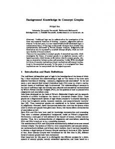
4. Experiments In this section, we present a case-study of our framework for worst-case disclosure using the Adult Database from the UCI Machine Learning Repository [26]. We only consider the projection of the Adult Database onto five attributes – Age, Marital Status, Race, Gender and Occupation. The dataset has 45,222 tuples after removing tuples with missing values. We treat Occupation as the sensitive attribute; its domain consists of fourteen values. We use pre-defined generalization hierarchies for the attributes similar to the ones used in [22]. Age can be generalized to six levels (unsuppressed, generalized to intervals of size 5, 10, 20, 40, or completely suppressed), Marital Status can be generalized to three levels, and Race and Gender can each either be left as is or be completely suppressed. We consider all the possible anonymized tables using those generalizations, ignoring those anonymizations that contained a bucket where all tuples had the same sensitive attribute, because such anonymizations lead to full disclosure without any additional background knowledge. All experiments were run under Linux (Ubuntu) on a machine with a 2.6GHz Intel Pentium 4 processor and 512MB of RAM. We computed the maximum disclosure for background knowledge ranging from zero pieces of knowledge (i.e., no background knowledge) to twelve pieces of knowledge for various bucketizations. Figure 5 plots, for one anonymized table, the number of pieces of knowledge available to an adversary against the maximum disclosure for both negated atoms (ℓ-diversity) and basic implications. In the anonymized table used, all the attributes other than Age were suppressed and the Age attribute was generalized to intervals of size 20. The solid line corresponds to implication statements and the dotted line corresponds to negated atoms. This graph agrees with our earlier observation that implication-type background knowledge subsumes negation; the maximum disclosure for k negated atoms is always smaller than the maximum disclosure for k implications. However, note that, for a given k, the difference between the maximum disclosure for negated atoms and for basic implications is not too large. One favorable outcome of this observation is that an anonymized table which tolerates maximum disclosure due to k negated atoms need not 5 While these algorithms typically have worst-case exponential running time in the height of the bucketization lattice, they have been shown to run fast in practice.

be anonymized much further to defend against k implications. Intuitively, if all the buckets in a table have a nearly uniform distribution, then the maximum disclosure should be lower, but the exact relationship is not obvious. To get a better picture, we performed the following experiment. We fixed a value k for the number of pieces of information. For every entropy value h, we looked at all tables T (h) for which the minimum entropy of the sensitive attribute over all buckets was equal to h. Amongst T (h) we found the table T (h) with the least maximum disclosure for k implications. Let the worst case disclosure for T (h) given k pieces of knowledge be denoted by w(T (h), k). We plotted h versus w(T (h), k) for k = 1, 3, 5, 7, 9, 11 in Figure 6. We see a behaviour which matches our intuition. For a given k, the disclosure risk monotonically decreases with increase in h. This is because increasing h means that we are looking at tables with more and more entropy in their buckets (and, consequently, less skew). We plotted an analogous graph (which we do not show here) for negation statements and observed very similar behaviour.

5. Related Work Publishing anonymous data involves trading off utility for privacy. Many metrics have been proposed to quantify the privacy guaranteed. ‘Perfect privacy’ [12, 25] guarantees that published data does not disclose any information about the sensitive data. However, checking whether a conjunctive query discloses any information about the answer to another conjunctive query is shown to be very hard (Πp2 complete [25]). Subsequent work showed that checking for perfect privacy can be done efficiently for many subclasses of conjunctive queries [23]. Perfect privacy places extremely strong restrictions on the types of queries that can be answered [25] (in particular, aggregate statistics cannot be published). Less restrictive privacy definitions based on asymptotic conditional probabilities [11] and certain answers [28] have been proposed. Statistical databases allow answering aggregates over sensitive values without disclosing the exact value [1]. Work on de-identification, like kanonymity [30] and “blending in a crowd” [8], ensures that an individual cannot be associated with a unique tuple in an anonymized table. However, under both of those definitions, sensitive information can be disclosed if groups are homogeneous. Background knowledge can lead to unwanted disclosure of sensitive information. Su et al. [29] and Yang et al. [33] limit disclosure in the presence of dependencies in the data known to the data publisher. The notion of ℓ-diversity [24] guards against limited amounts of background knowledge unknown to the data publisher. Farkas et al. [16] provide a survey of indirect data disclosure via inference channels.

1

1 implication negation

number of implications = 1 number of implications = 3 number of implications = 5 number of implications = 7 number of implications = 9 number of implications = 11

0.9 0.9 0.8

min worst case disclosure

max disclosure

0.8

0.7

0.6

0.7

0.6

0.5

0.4

0.5 0.3 0.4 0.2

0.3

0.1 0

2

4

6 number of conjuncts

8

10

12

Figure 5. Disclosure vs # pieces of background knowledge There are several approaches to anonymizing a dataset to ensure privacy. These include generalizations [7, 22, 27], cell and tuple suppression [9, 27], adding noise [1, 5, 8, 15], publishing marginals that satisfy a safety range [14], and data swapping [10] - a technique where attributes are swapped between tuples in such a way that certain marginal totals are preserved. Queries can also be posed online and the answers audited [20] or perturbed [13]. Not all approaches guarantee privacy. For example, adding uncorrelated random noise to the attributes in a tuple is not sufficient to ensure privacy. Spectral techniques can be used to separate much of the noise from the data [17, 19]. Anatomy [32] is a recently proposed technique for anonymizing a dataset. It corresponds to exactly to the notion of bucketization that we use in this paper. When the attacker knows full identification information, then generalization provides no more privacy than bucketization. In practice, however, we recommend generalizing the attributes in the buckets before publishing the data for the following reasons. It is very rare for an attacker to actually have full identification information. Thus disclosing the precise values of the non-sensitive attributes will allow an attacker to use linking attacks [30] to identify individuals in the anonymized table. In many cases, the fact that a particular individual is in the table is considered sensitive information [8]. Furthermore, certainty that an individual is in the table leads to more precise inference about sensitive values than uncertainty about the presence of the individual. The utility of data that has been altered to preserve privacy has often been studied in contexts where the future use of the data is known. Examples of such work are methods to reconstruct association rules [15], distributions of continuous variables [3, 5] from noisy data; methods to perturb the values of continuous numeric attributes so that data clusters can be reconstructed [8]; and methods to anonymize data while trying to maximize decision tree accuracy [18, 31]. There have also been some negative results for utility. Publishing a single k-anonymous table has been shown to be

1

1.2

1.4

1.6 1.8 min entropy

2

2.2

2.4

Figure 6. Entropy vs Maximum Disclosure Risk affected by the curse of dimensionality [2]; large portions of the data are required to be suppressed to ensure privacy. Subsequent work [21] shows how to publish several tables instead of a single one to combat this curse.

6. Conclusions In this paper, we initiate a formal study of the worstcase disclosure risk with background knowledge. Critically, our analysis does not assume that we are aware of the exact background knowledge possessed by the attacker. We only assume bounds on the the attacker’s background knowledge in terms of the number of basic units of knowledge that the attacker possesses. We propose basic implications as an expressive and natural choice for these basic units of knowledge. Although computing the probability of disclosure associated with a specific set of k basic implications is intractable, we show how to efficiently determine the worst-case over all sets of k basic implications. In addition to assessing maximum disclosure, we show how to search for a bucketization that is robust (to a desired threshold) against any k units of knowledge by incorporating the check for (c, k)-safety into existing lattice-search algorithms. Finally, we demonstrate that, in practice, ℓ-diversity has similar maximum disclosure risk to our notion of (c, k)-safety, which guards against a richer class of background knowledge. In this paper we choose basic implications as our units of knowledge so that we can express any background knowledge. It is clear that our algorithms yield extremely conservative bucketizations if we try to protect against an attacker who knows information that can only be expressed using a large number of basic implications. Since basic implications are essentially CNF clauses with at least one negative atom, our language suffers from an exponential blowup in the number of basic units required to express arbitrary DNF formulas. Other choices of basic units may lead to equally expressive languages while at the same time requiring fewer

basic units to express certain natural properties. One approach to reducing the number of basic units required to express a property is to add more powerful atoms to our existing language. For example, an interesting class of DNF formulas are those of the form

[14] A. Dobra. Statistical tools for disclosure limitation in multiway contingency tables. PhD thesis, Carnegie Mellon University, 2002.

∨s∈S (tp [S] = s ∧ tp′ [S] = s)

[16] C. Farkas and S. Jajodia. The inference problem: a survey. SIGKDD Explor. Newsl., 4(2), 2002.

Such formulas express equality between the sensitive attributes of two tuples and can be expressed using |S| basic implications. Finding the right choice of basic units of knowledge is an important direction of future work. Other directions for future work include extending our framework to allow for probabilistic background knowledge, studying cost-based disclosure (since it was observed in [24] that not all disclosures are equally bad), and finally extending our results to other forms of anonymization beyond bucketization and generalization, such as dataswapping and collections of anonymized marginals [21].

[17] Z. Huang, W. Du, and B. Chen. Deriving private information from randomized data. In SIGMOD, 2004.

References [1] N. R. Adam and J. C. Wortmann. Security-control methods for statistical databases: a comparative study. ACM Comput. Surv., 21(4):515–556, 1989. [2] Charu C. Aggarwal. On k-anonymity and the curse of dimensionality. In VLDB, pages 901–909, 2005. [3] D. Agrawal and C. C. Aggarwal. On the design and quantification of privacy preserving data mining algorithms. In PODS, 2001. [4] R. Agrawal and R. Srikant. Fast algorithms for mining association rules in large databases. In VLDB, 1994. [5] R. Agrawal and R. Srikant. Privacy preserving data mining. In SIGMOD, 2000. [6] F. Bacchus, A. J. Grove, J. Y. Halpern, and D. Koller. From statistical knowledge bases to degrees of belief. A.I., 87(1-2), 1996. [7] R. J. Bayardo and R. Agrawal. Data privacy through pptimal k-anonymization. In ICDE, 2005. [8] S. Chawla, C. Dwork, F. McSherry, A. Smith, and H. Wee. Toward privacy in public databases. In TCC, 2005. [9] L. H. Cox. Suppression, methodology and statistical disclosure control. Journal of the American Statistical Association, 75, 1980. [10] T. Dalenius and S. Reiss. Data swapping: a technique for disclosure control. Journal of Statistical Planning and Inference, 6, 1982. [11] N. Dalvi, G. Miklau, and D. Suciu. Asymptotic conditional probabilities for conjunctive queries. In ICDT, 2005. [12] A. Deutsch and Y. Papakonstantinou. Privacy in database publishing. In ICDT, 2005. [13] I. Dinur and K. Nissim. Revealing information while preserving privacy. In PODS, pages 202–210, 2003.

[15] A. Evfimievski, J. Gehrke, and R. Srikant. Limiting privacy breaches in privacy preserving data mining. In PODS, 2003.

[18] Vijay S. Iyengar. Transforming data to satisfy privacy constraints. In KDD, pages 279–288, 2002. [19] H. Kargupta, S. Datta, Q. Wang, and K. Sivakumar. On the privacy preserving properties of random data perturbation techniques. In ICDM, pages 99–106, 2003. [20] K. Kenthapadi, N. Mishra, and K. Nissim. Simulatable auditing. In PODS, 2005. [21] Daniel Kifer and Johannes Gehrke. Injecting utility into anonymized datasets. In SIGMOD, 2006. [22] K. LeFevre, D. DeWitt, and R. Ramakrishnan. Incognito: Efficient fulldomain k-anonymity. In SIGMOD, 2005. [23] A. Machanavajjhala and J. Gehrke. On the efficiency of checking perfect privacy. In PODS, 2006. [24] A. Machanavajjhala, J. Gehrke, D. Kifer, and M. Venkitasubramaniam. ℓ-diversity: Privacy beyond k-anonymity. In ICDE, 2006. [25] G. Miklau and D. Suciu. A formal analysis of information disclosure in data exchange. In SIGMOD, 2004. [26] U.C. Irvine Machine Learning Repository. http://www.ics.uci.edu/ mlearn/mlrepository.html. [27] P. Samarati and L. Sweeney. Protecting privacy when disclosing information: k-anonymity and its enforcement through generalization and suppression. Technical report, CMU, SRI, 1998. [28] K. Stoffel and M. Studer. Provable data privacy. In DEXA, 2005. [29] T. Su and G. Ozsoyoglu. Controlling fd and mvd inferences in multilevel relational database systems. IEEE TKDE, 3(4), 1991. [30] L. Sweeney. k-anonymity: a model for protecting privacy. International Journal on Uncertainty, Fuzziness and Knowledge-based Systems, 10(5):557–570, 2002. [31] K. Wang, B. C. M. Fung, and P. S. Yu. Template-based privacy preservation in classification problems. In ICDM, November 2005. [32] X. Xiao and Y. Tao. Anatomy: Simple and effective privacy preservation. In To appear in VLDB, 2006. [33] X. Yang and C. Li. Secure xml publishing without information leakage in the presence of data inference. In VLDB, pages 96–107, 2004.

A Completeness Proof of Theorem 3 Since the attacker is assumed to have full identification information, the values of tp [X] and which bucket tp falls into are assumed to be common knowledge. The only remaining information that it takes to completely define a particular table is the mapping between people and sensitive values within each bucket. Thus we need to show that a finite conjunction of basic implications can express any set of mappings between people in the table and sensitive values. Note that, since the domain of S and the table size are finite, there are only finitely many mappings between people in the table and sensitive values. Any particular such mapping between people and sensitive values can clearly be represented by a finite conjunctions of atoms of the form tp = s. Thus any set of mappings between people and sensitive values can be represented by a finite disjunction of finite conjunctions of atoms. We show that, in fact, a finite conjunction of basic implications can represent any finite boolean combination of atoms. Consider any finite boolean combination of atoms. Without loss of generality, assume that the formula is in conjunction normal form. It thus remains to show that any disjunction of literals (i.e., atoms or their negations) can be representated by a finite conjunction of basic implications. We break this into two cases dependeing on whether or not the given disjunction contains at least one negative literal. In the first case, if the disjunction contains at least one negative literal, then the disjunction is equivalent to a single a basic implication ϕ → θ where ϕ is the conjunction of the atoms appearing in the negative literals and ψ is the conjunction of the atoms appearing in the positive literals. In the second case, if the disjunction contains no negative literals, the disjunction is equivalent to the following conjunction of basic implications: ∧s∈S (tp = s → ϕ), where ϕ is the given disjunction itself and p is any person in the table. 

B Hardness Proof of Theorem 8 Consider the problem of deciding if B and ϕ are both satisfiable by some table T , given as input a bucketization and a conjunction of simple implications. It is clear that the problem is in NP, because given a mapping of tuples to sensitive values (which has a description that is linear in bucketization size), we can verify that it is indeed consistent with the bucketization and that it satisfies ∧i∈[k] (Ai → Bi ) in polynomial time. To show that the problem is NP-hard, we reduce the problem of deciding 3-CNF satisfiability, which is NPcomplete, to this problem as follows. Consider any 3-CNF formula. We construct a bucketization and set of basic implications from this formula as follows. For each variable x mentioned in the 3-CNF formula, we construct a bucket

containing two tuples, named tx and t¬x , and two sensitive values, T and F . For each clause C of the form X ∨ Y ∨ Z in the 3-CNF formula (where X, Y, Z are either variables or their negations), we construct a bucket containing five tuC C C C ples, named tC X , tY , tZ , tdummy1 , tdummy2 , and five sensitive values, T, T, T, F, F . The background knowledge then consists of the following set of statements: • tx [S] = T → tC X [S] = T , for every variable x and every clause C containing literal X ≡ x, • tC X [S] = T → tx [S] = T , for every variable x and every clause C containing literal X ≡ x, • t¬x [S] = T → tC X [S] = T , for every variable x and every clause C containing literal X ≡ ¬x, • tC X [S] = T → t¬x [S] = T , for every variable x and every clause C containing literal X ≡ ¬x, and C • tC dummy1 [S] = T → tdummy2 [S] = T , for every clause C.

Let k be the number of implications that we added above. Note that k is linear in the size of the 3-CNF formula. It is fairly clear that if there is a mapping of tuples to values that is consistent with the bucketization and background knowledge, then assigning each variable x to the value tx [S] satisfies the 3-CNF formula (since, in each bucket corresponding to a clause, at least one tuple representing a literal must have sensitive value T ). So we can decide if the 3-CNF formula is satisfiable, given an oracle for our problem. Thus the decision problem is NP-complete. It should therefore not come as a surprise that computing the probability of Pr(C | B ∧ (∧i∈[k] (Ai → Bi ))) is #Pcomplete since computing the probability and counting satisfying assignments are intimately related. We reduce the problem of counting the satisfying assignments of a 2-CNF formula, which is #P-complete [?], to an instance of computing Pr(A | B ∧ (∧i∈[k] (Ai → A′i ))). Consider a 2-CNF formula ϕ, with variables x0 , . . . , xn−1 . We can find a satisfying assignment of ϕ in polynomial time since ϕ is 2-CNF. Let ∧i∈[n] Xi represent the satisfying assignment, where Xi is either xi or ¬xi , depending on the value of xi in the satisfying assignment. Consider a complete binary tree with n leaf nodes, where the ith leaf is associated with the literal Xi . For every non-leaf node, we introduce a new variable y and a constant number of 3-CNF clauses that are equivalent to y ↔ U ∧ V , where U and V are the literals at the left and right children of the non-leaf node. Let ϕ′ be the conjunction of all the newly-introduced 3-CNF clauses. Then the conjunction of all the newly-introduced 3-CNF clauses implies that y ↔ ∧i∈[n] Xi . Note that ϕ′ is polynomial in the size of ϕ since the complete binary tree with n leaves has at most O(n) nodes, and we introduced a constant number of clauses for each internal node. ϕ ∧ ϕ′ is 3-CNF formula.

And ϕ ∧ ϕ ∧ y is a 3-CNF formula with exactly one satisfying assignment (namely, setting each variable in ϕ according to ∧i∈[n] Xi , and each newly-introduced variable to true). So, applying the construction from the proof of Theorem 8 to get A and Ai from ϕ ∧ ϕ′ , it is easy to check that 1 Pr(ty [S]=T |ϕB ∧ϕ∧ϕ′ ) is exactly the number of satisfying assignments of ϕ. 

′ Lemma 16 For all θ0 , . . . , θk−1 , θ0′ , . . . , θk−1 , ψ, ϕ, such ′ that θi → θi , for all i ∈ [k], we have

Pr(ϕ | ψ ∧ (∧i∈[k] (θi → ϕ))) ≤ Pr(ϕ | ψ ∧ (∧i∈[k] (θi′ → ϕ))). Proof

Pr(ϕ | (∧i∈[k] (θi → ϕ)) ∧ ψ) Pr((∧i∈[k] (θi →ϕ))∧ψ∧ϕ) = Pr((∧i∈[k] (θi →ϕ))∧ψ)

It is prudent at this point to mention that we have a notion of independence between buckets for the general language.

Pr(ϕ∧ψ) 1−Pr(∨i∈[k] (θi ∧¬ϕ)∨¬ψ) .

=

So it is enough if we show that

C Special Form for Maximum Disclosure Proof of Lemma 10 For convenience of notation, • let θ be ¬(∧i∈[k] ¬θi ), • let χ be (∧i∈[k] (θi → ϕi )), • let u = Pr(θ ∧ ϕ ∧ ψ), • let v = Pr(¬θ ∧ ψ ∧ ϕ), • let w = Pr(¬θ ∧ ψ), • let x = Pr(θ ∧ χ ∧ ψ ∧ ϕ), and

Pr(∨i∈[k] (θi ∧ ¬ϕ) ∨ ¬ψ) ≤

We know that θi → θi′ . Hence, any model that satisfies θi also satisfies θi′ . This implies that any model that satisfies (∨i∈[k] (θi ∧¬ϕ)∨¬ψ) also satisfies (∨i∈[k] (θi′ ∧¬ϕ)∨¬ψ). Hence, the required result.  Proof of Lemma 12 max

atoms A,Ai

=

• let y = Pr(θ ∧ χ ∧ ψ). Then, for all ψ ′ ∈ L, ∧i∈[k] (θi → ϕ) ∧ ψ ′ is logically equivalent to (θ ∧ ϕ ∧ ψ ′ ) ∨ (¬θ ∧ ψ ′ ). Hence, Pr(ϕ | (∧i∈[k] (θi → ϕ)) ∧ ψ) Pr((∧i∈[k] (θi →ϕ))∧ψ∧ϕ) = Pr((∧i∈[k] (θi →ϕ))∧ψ) = = =

Pr((θ∧ϕ∧ϕ∧ψ)∨(¬θ∧ψ∧ϕ)) Pr((θ∧ϕ∧ψ)∨(¬θ∧ψ)) Pr(θ∧ϕ∧ψ)+Pr(¬θ∧ψ∧ϕ) Pr(θ∧ϕ∧ψ)+Pr(¬θ∧ψ) u+v u+w .

Similarly, using that fact that, for all ψ ′ ∈ L, ∧i∈[k] (θi → ϕi ) ∧ ψ ′ is logically equivalent to (θ ∧ χ ∧ ψ ′ ) ∨ (¬θ ∧ ψ ′ ), we get:

Pr(∨i∈[k] (θi′ ∧ ¬ϕ) ∨ ¬ψ).

= = =

Pr(A | B ∧ (∧i∈[k] Ai → A))

max

Pr(A ∧ (∧i∈[k] (Ai → A)) | B) Pr((∧i∈[k] (Ai → A)) | B)

max

Pr(A | B) Pr(¬A ∧ (∧i∈[k] ¬Ai ) ∨ A | B)

atoms A,Ai

atoms A,Ai

max

atoms A,Ai

max

Pr(A | B) Pr(¬A ∧ (∧i∈[k] ¬Ai ) | B) + Pr(A | B) 1

atoms A,Ai Pr(¬A∧(∧i∈[k] ¬Ai )|B) Pr(A|B)

+1

Hence the required result.  Proof of Lemma 13 When Ai,j is tpi = sjb for all i ∈ [l] and all j ∈ [ki ], then it is easy to see that P Y nb − i − j∈[ki ] nb (sjb ) Pr(∧i∈[l],j∈[ki ] ¬Ai,j | B) = . nb − i i∈[l]

Pr(ϕ | (∧i∈[k] (θi → ϕi )) ∧ ψ) = Pr(θ∧χ∧ψ∧ϕ)+Pr(¬θ∧ψ∧ϕ) Pr(θ∧χ∧ψ)+Pr(¬θ∧ψ) x+v . = y+w However, since θ ∧ χ ∧ ψ ∧ ϕ logically implies both θ∧ϕ∧ψ and θ∧χ∧ψ, we have u ≥ x and y ≥ x. Similarly, since ¬θ ∧ ψ ∧ ϕ logically implies ¬θ ∧ ψ, we have v ≤ w. u+v x+v x+v So, since u, v, w, x, y ≥ 0, we get u+w ≥ x+w ≥ y+w , thus proving the required result.  Proof of Lemma 11 Since each of the implications (θi → B) is basic, θi is a conjunction of positive atoms. Hence, from each of the θi pick one of the atoms Ai (the atoms need not be distinct). Clearly, θi → Ai . Hence, the required result follows from Lemma 16. 

We now show, by induction on l (i.e., the number of people involved in the k atoms), that for all b ∈ B and all atoms Ai,j (not necessarily ti [S] = si ) such that Ai,j and Ai,j ′ mention the same tuple in b iff i = i′ , we have P Y nb − i − j∈[ki ] nb (sjb ) . Pr(∧i∈[l],j∈[ki ] ¬Ai,j | B) ≥ nb − i i∈[l]

In the base case (i.e., l = 1, k0 = k), all the atoms mention the same person, say p0 . So taking A0,j to be tp0 [S] = sjb for j ∈ [k] clearly minimizes Pr(∧j∈[k] ¬A0,j | B), and n −Σ

n (sj )

b b actually achieves a probability of b j∈[k] . nb Suppose that the induction hypothesis holds for all l. Consider the case for l+1. Consider p0 , the person involved

in the most (i.e., k0 ) atoms (namely, A0,j , for j ∈ [k0 ]). Let S ′ be the set of values in S not involved in these atoms. That is, S ′ = {s ∈ S : ∀j ∈ [k0 ] . A0,j 6≡ tp0 [S] = s}. For each s ∈ S ′ , • let kis = ki+1 , for each i ∈ [l], • let Asi,j be Ai+1,j for each i ∈ [l] and each j ∈ [kis ], • let bs and B s be the bucket and bucketization, respectively, obtained from b and B by removing tp0 [X] and one occurrence of s from b. Then it is easy to see that • nbs = nb − 1, P P j j • j∈[ki+1 ] nb (sb ) j∈[ks ] nbs (sbs ) ≤ i

So, using these facts and the induction hypothesis, we get: Pr(∧i∈[l+1],j∈[k ¬Ai,j | B) i] P = (Pr(∧ ′ i∈[l+1],j∈[ki ] ¬Ai,j | B ∧ tp0 [S] = s) s∈S × Pr(tp0 [S] = s | B)) P s s nb (s) Pr(∧ = ′ i∈[l],j∈[kis ] ¬Ai,j | B ) nb s∈S P nbs −i− j∈[ks ] nbs (sjbs ) n (s) Q P i ) bnb ( ≥ ′ i∈[l] s∈S nP bs −i j nb (sb ) n (s) nb −i−1− j∈[k Q P i+1 ] ≥ ) bnb s∈S ′ ( i∈[l] P nb −i−1 j nb (sb ) P nb −i−1− j∈[k Q i+1 ] ) s∈S ′ nnb (s) = ( i∈[l] nP b −i−1 b P nb −i−1− j∈[k nb (sjb ) nb − j∈[k ] nb (sjb ) Q i+1 ] 0 ) ≥ ( i∈[l] nb −i−1 nb P Q nb −i− j∈[k ] nb (sjb ) i = i∈[l+1] nb −i This completes the induction. 

D Monotonicity Proof of Theorem 15 Let b1 and b2 be two buckets of sizes m and n respectively in bucketization B. Let b be the bucket formed by merging b1 and b2 and let B ′ be the new bucketization. To show monotonicity, it is enough to show that the minimum Pr(∧i∈[k] ¬Ai | B) is at least as much as the minimum Pr(∧i∈[k] ¬Ai | B ′ ) where Ai range over atoms that involve only people in b in both cases. According to Lemma 13, let tpi [S] = sjb be the atoms that minimize the second probability (for B ′ ), for i ∈ [l] and j ∈ [ki ] (where p0 , . . . , pl are the people involved in k0 , . . . , kl atoms, respectively). Then, as in Lemma 13, the minimum probability is given by: Y ai + b i − i i∈[l]

m+n−i

P where ai := nb1 − j∈[i] nb1 (sjb ) and bi = nb2 − P j j∈[i] nb2 (sb ). For each i, we inductively define Pi , ci , and di as follows:

1. P0 = 1, c0 = 0, d0 = 0. i −ci i −di i −ci 2. If am−c ≤ bn−d then Pi+1 = Pi am−c and ci+1 = i i i ci + 1 and di+1 = di . i −ci i −di i −di 3. If am−c > bn−d then Pi+1 = Pi bn−d and ci+1 = ci i i i and di+1 = di + 1.

Think of this as choosing atoms tp′i = sjb for i ∈ [l], j ∈ [ki ] where p′i is a new person in bucket b1 or b2 depending on i −di−1 i −ci−1 ≤ bn−d or not. It is easy to see that whether am−c i−1 i−1 Pl ≤ P (∧i∈[l],j∈[ki ] ¬tp′i = sjb | B). Note that, by defi +bi −i inition, ci + di = i for all i. So we have am+n−i = m−ci ai −ci ni −di bi −di ai −ci +bi −di m−ci +n−di = m−ci +n−di m−ci + m−ci +n−di n−di ≥ i −ci bi −di , n−di ). So at each step i, we get Pi+1 by mulmin( am−c i i +bi −i . So tiplying Pi by a factor that is no more than am+n−i Q j ai +bi −i Pl ≥ i∈[l] m+n−i Thus P (∧i∈[l],j∈[ki ] ¬tp′i = sb | B) ≥ Q ai +bi −i i∈[l] m+n−i and so we are done. 

E Maximum Disclosure and ℓ-diversity We now use our framework to analyze a different restriction on background knowledge and relate this with a privacy condition recently proposed in [24], called ℓ-diversity. This exercise provides further insight into our techniques, while at the same time contributing an essential piece of formal analysis that was missing in [24], namely, proving that rec cursive (c, ℓ)-diversity is equivalent to ( c+1 , ℓ − 2)-safety with respect to a simple language expressing sensitive value elimination. This is an important contribution to our understanding of (c, ℓ)-diversity because it shows that (c, ℓ) diversity protects against ℓ − 2 pieces of information involving possibly several different people, rather than the earlier belief that it protects against ℓ − 2 pieces of information involving only one person. Before we begin, however, let us quickly recall the definition of recursive (c, ℓ)-diversity. Definition 17 (Recursive (c, ℓ)-diversity) A bucketization B is said to be recursive (c, ℓ)-diverse if for all buckets b ∈ B, ℓ−2 X nb (sib )) nb (s0b ) ≤ c × (nb − nb (s0b ) − i=1

Intuitively, this definition states that a bucketization is (c, 2)-diverse if for every bucket, the most frequent attribute value of the sensitive attribute appears at most c times as frequently as all the remaining attribute values of the sensitive attribute combined. As argued in [24], it then follows that if an adversary is able to eliminate k − 2 values of the sensitive attribute of one particular individual in some bucket, c the disclosure risk for that individual is at most c+1 .

We now show that eliminating the sensitive values for one particular individual maximizes disclosure over background knowledge from language Lneg (defined below), which allows for sensitive value elimination for possibly several different individuals. Once again the disclosure maximizing background knowledge has a special structure, namely, that all statements mentioned the same tuple. Our proof uses the techniques from Section 3. Definition 18 Let Lneg be the set of the formulas of the form ¬A where A is an atom. Recall that an atom is a formula of the form tp [S] = s. Lneg thus captures knowledge of the form “Ed does not have the flu”. Theorem 19 For any bucketization B, we have maxatoms A,Ai Pr(A | B ∧ (∧i∈[k] ¬Ai )) n (s0 ) = maxb∈B n −P b bn (si+1 ) b

i∈[k]

b

b

Proof This follows immediately from independence between the permutations in separate buckets and Lemma 20 below.  Lemma 20 Consider a bucket b ∈ B, and let p be any person with a tuple tp in b. Then Pr(A | B ∧ (∧i∈[k] ¬Ai )) is maximized over all atoms A, A0 , . . . , Ak−1 that involve only people from b when 1. A is tp [S] = s0b , and 2. Ai is tp [S] = si+1 b , for i ∈ [k]. Moreover, the maximum probability is given by nb (s0b ) P nb − i∈[k] nb (si+1 b ) Proof First note that when A is the statement tp [S] = s0b , and each Ai is the statement tpi [S] = si+1 b , then it is easy to see that Pr(A | B ∧ (∧i∈[k] ¬Ai )) =

nb (s0b )

nb −

P

i∈[k]

nb (si+1 b )

(3)

since this is the relative frequency of s0b after s1b , . . . , skb have been eliminated. We now show that no other choice of atoms A, Ai (involving only people with tuples in b) gives a higher probability. We proceed by induction on the number of people involved in the atoms A0 , . . . , Ak−1 to show that Pr(A | B ∧ (∧i∈[k] ¬Ai )) ≤

nb (s0b ) P nb − i∈[k] nb (si+1 b )

In the base case, where all the atoms A, A0 , . . . , Ak−1 involve exactly one person, it is easy to see that the worst

case is given by Equation 3. Now, using the induction hypothesis, assume that the Lemma is true when the atoms involve at most m − 1 distinct people. We will consider the case where A, A0 , . . . , Ak−1 involve m ≥ 2 people. Let p be the person involved in A. Now A0 , . . . , Ak−1 involve some other person p′ 6= p, since m ≥ 2. Without loss of generality, A0 , . . . , Ak′ −1 be the atoms not involving p′ and let Ak′ , . . . , Ak−1 be the atoms involving p′ , for some k ′ < k. For ease of notation, we abbreviate ∧i∈[k] ¬Ai by κ and ∧i∈[k′ ] ¬Ai by κ′ . Thus our original background knowledge κ is split into two parts. The first part, κ′ , is the part of our background knowledge not involving p′ ; the second part, ∧i∈[k]\[k′ ] ¬Ai , is the part of our background knowledge involving only p′ . Since k ′ < k, we can apply our induction hypothesis to the statement κ′ . Let Sb be the set of sensitive values that appear in bucket b (i.e., Sb = {s ∈ S : nb (s) > 0}). For each s ∈ Sb , let bs and B s be the bucket and bucketization, respectively, that are obtained by removing the non-sensitive attributes of p′ and an occurrence of s from bucket b. Then it is not hard to show that: • nbs = nb − 1, • nbs (s0bs ) ≤ nb (s0b ), and P P i+1 • 1 + i∈[k′ ] nbs (si+1 i∈[k] nb (sb ) bs ) ≤ So, using the induction hypothesis (in the first inequality below) and the above facts (in the second inequality), we get Pr(A | P B ∧ κ) = Ps∈Sb Pr(A ∧ tp′ [S] = s | B ∧ κ) = s∈Sb Pr(A | B ∧ κ ∧ tp′ [S] = s) × Pr(tp′ [S] = s | B ∧ κ) P Pr(A | B s ∧ κ′ ) Pr(tp′ [S] = s | B ∧ κ) = Ps∈Sb nbs (s0bs ) ≤ i+1 Pr(tp′ [S] = s | B ∧ κ) s∈Sb nbs −P s i∈[k′ ] nb (sbs ) 0 P nb (sb ) ≤ i+1 Pr(tp′ [S] = s | B ∧ κ) s∈Sb nb −P ) i∈[k] nb (sb 0 P nb (sb ) = n −P s∈Sb Pr(tp′ [S] = s | B ∧ κ) n (si+1 ) b

≤

i∈[k]

b

b

n (s0 ) P b b ) nb − i∈[k] nb (si+1 b

This completes the induction.