Abstract. Values far from the center of the data are called outliers. These can be highly influential in determining the character of descriptive statistics.
SD01
Using Biweights for Handling Outliers George W. Dombi, PhD., Karmanos Cancer Center, Detroit, MI Abstract Values far from the center of the data are called outliers. These can be highly influential in determining the character of descriptive statistics. M-estimators are a class of central tendency measures than replace the mean and are highly resistant to local misbehavior caused by outlier data. Beaton and Tukey introduced the biweight as an iteratively reweighed measure of central tendency. Huber also introduced a different but complementary M-estimator. SAS will calculate both the biweight and the Huber weight function in Proc Stdize. Proc Nlin will allow for biweight and Huber weights to be utilized in user developed equations. Introduction In real data, some values are very different from the bulk of the data. Values far from the center of the data can be highly influential in determining the character of descriptive statistics. The mean is sensitive to outliers; for example: Case 1: {2, 3, 4, 5, 6} mean = 4 Case 2: {2, 3, 4, 5, 67} mean = 16.2 In Case 2, the value 67 is an outlier. It pulls the mean to a value of 16.2 which is outside the bulk of the remaining data. Terms like resistant and robust are often used to describe measures that are not so easily affected by outliers. For the purpose of this report, the term resistant will be assigned to descriptive statistics and the term robust will be assigned to inferential statistics. Thus, resistant descriptive statistics are insensitive to local misbehavior caused by outlier data. While robust inferential statistics are tolerant to departures from the assumptions of normal distributions. The mean is not a resistant descriptive statistic. The T-test is not a robust inferential statistic because it relies heavily on the mean. One the other hand, the median is a resistant measure of central tendency. One can see that the median is resistant to outliers since it completely ignores extreme values. Case 1: {2, 3, 4, 5, 6} median = 4 Case 2: {2, 3, 4, 5, 67} median = 4 The Anova test, which relies more heavily on the standard deviation, is more robust than the t-test. The concept of weighing data points relative to their distance from the center of the data set is an idea that is more widely accepted. Weighing is already in use but not acknowledged. The mean can be thought of using a weight equal to 1 for each data point. On the other hand, the median uses a weight of 0 for each rank ordered data point then uses weight equal 1 for the center most data. What if you want to use a range a weights varying from 0 to 1 with respect to the distance from the center of the data? How would you determine these intermittent
values of weight? This is part of the motivation for creating the M-estimators. Mestimators are a class of central tendency measures that have variable weight for each datum. Notice the continuation of the letter ‘M’; Mean, Median, and M-estimators are all measures of central tendency. M-estimators usually provide greater weight for data values near the center of the data cluster and decreasing weight for data away from the center. M-estimators are sometimes denoted by the Greek letter theta, Θ, and are set equal to the sum of (weight *individual data value) / sum of weights. M-estimator = Θ = Σwi*xi Σwi Xi = numbers Wi = weights 0 … 1 Where Θ is iteratively refined by: (xi – Θ) = u δ δ = MAD (median absolute deviation) u = parameter descriptor that defines individual M-estimator. In 1974, Albert Beaton and John Tukey introduced the concept of an iterative reweighed measure of central tendency, called the biweight, as an abbreviation for bisquare weight. The biweight is an M-estimator that satisfies the definitions given above and the weight is calculated as: weight = weight =
{1-(u^2)/4.685^2}^2 0
when abs(u) 4.685
This is not a very pretty picture in the way the biweight is shown but you can see the square of the square that gives it its name. The cut off point is a user selected value that is most often in the range of 4-6. In this case the cut point is 4.685, where the weight becomes zero. The biweight is considered to be robust since it is not sensitive to outlier data. Biweight depends on the calculated weights and the weights depend on the biweight so we need an iterative solution. Once calculated, the M-estimator becomes the new measure of central tendency for the next iteration. Figure 1 shows the weight at various values of u. Note that when the difference between the data point and the M-estimator (in this case the biweight) is small, then the weight equals 1. Then as the difference increase, as u increases, the value of the biweight declines. For differences larger than 4.65 the biweight equals zero.
2
Tukey Bisquared Weight 1.2
Weight
1 0.8 Tukey Bisquared Weight
0.6 0.4 0.2 0 -6 -5 -4 -3 -2 -1 0
1
2
3
4
5
6
U value
Figure 1. Biweight function decreases to 0 as distance of data point increases away from the middle of the data set. Another kind of M-estimator is the Huber weight. This also needs a user selected cutoff point. Huber weights never go completely to zero and some people like that because it is easier to integrate as a continuous function. Often the Huber weight and the biweight are used in the same calculation. The Huber weight is utilized first to get near the convergence point and then use the biweights to get a discrete value cut off of zero for the outlier data.
3
Huber Weight 1.2 1 Weight
0.8 0.6
Huber Weight
0.4 0.2 0 -6
-5
-4
-3
-2
-1
0
1
2
3
4
5
6
U value
Figure 2. Huber weight function smoothly decreases, but not to 0, as the distance of a data point increases away from the middle of the data set. Where is the biweight used? An application from Affymetrix is presented below in which genomic data is being calculated using a single step biweight procedure to reduce noise between pairs of data. Afflymetrix uses the single step method as a compromise between need for real time speed versus accuracy of the calculation. To calculate the single-step biweight, the median is first determined from replicates as the measure of central tendency. S, the median absolute deviation, MAD, of the replicates is then calculated as a measure of spread in the data. U combines the median, the cutoff value c and the MAD to form the bisquared weight, Wi Note the use of epsilon to keep the denominator from equaling 0 and blowing-up the equation. Wi is the weight for each point. Finally the tukey biweight is calculated as the sum of the weights*data / sum of the weights as the new measure of the center. This method is supposed to be accurate to at least 80% depending on the spread in the replicates. With little spread the method is 100% equivalent to the fully iterated biweight calculation. z One-Step Tukey’s Biweight (implemented in Affymetrix software package): z The probe pair vote is weighted more strongly if this probe pair Signal value is closer to the median value for a probe set. z
tukey.biweight