A Modified Approach for Detection of Outliers

A Modified Approach for Detection of Outliers Iftikhar Hussain Adil Department of Economics School of Social Sciences and Humanities National University of Sciences and Technology Islamabad [email protected]

Ateeq ur Rehman Irshad Department of International Business &Marketing Nust Business School National University of Sciences and Technology Islamabad [email protected]

Abstract Tukey’s boxplot is very popular tool for detection of outliers. It reveals the location, spread and skewness of the data. It works nicely for detection of outliers when the data are symmetric. When the data are skewed it covers boundary away from the whisker on the compressed side while declares erroneous outliers on the extended side of the distribution. Hubert and Vandervieren (2008) made adjustment in Tukey’s technique to overcome this problem. However another problem arises that is the adjusted boxplot constructs the interval of critical values which even exceeds from the extremes of the data. In this situation adjusted boxplot is unable to detect outliers. This paper gives solution of this problem and proposed approach detects outliers properly. The validity of the technique has been checked by constructing fences around the true 95% values of different distributions. Simulation technique has been applied by drawing different sample size from chi square, beta and lognormal distributions. Fences constructed by the modified technique are close to the true 95% than adjusted boxplot which proves its superiority on the existing technique.

Keywords: Boxplot, Skewness, Medcouple, Adjusted boxplot, Modified Boxplot. 1. Introduction Tukey’s (1977) technique is used to detect outliers in univariate distributions for symmetric as well as in slightly skewed data sets. This technique constructs fence around the data leaving some observations on either side of the data which are treated as outliers. As the symmetry of the distribution decreases its performance worsens and it starts to construct fence which exceed from the data limit on one side and leaving some portion on the other side of the data. e.g. if the distribution is left skewed the upper fence exceeds from the maximum of the data and may ignore outliers while lower fence will identify lot of observation as outlier which are not outliers. Hubert and Vandervieren (2008) tried to overcome the problem by incorporating a robust measure of skewness in Tukey’s technique. G. Brys et. al. (2004) introduced “Medcouple” a robust measure of skewness and Hubert and Vandervieren incorporated it as a power of exponential times some constant on left and right as -3.5 and 4 changing position depending upon sign of medcouple. Incorporating this function, it condenses the interval from narrow side and extends the interval towards the puffy tail. It functions very Pak.j.stat.oper.res. Vol.XI No.1 2015 pp91-102

Iftikhar Hussain Adil, Ateeq ur Rehman Irshad

well as the distributions are highly skewed (skewness ≥3) but fails to work when the skewness is slightly less than 3. It constructs fence even larger than extremes of the data also leaving a great space between true values (2.5% and 97.5% of the distribution) and the fence constructed by it. Performance of adjusted box plot depends more on the exponential function relative to medcouple. This exponential function is multiplied on both sides with inter quartile range (IQR). Medcouple is a small number which remains generally in between 0.4 and 0.6 in absolute terms and cannot affect the constant multiplied by it as a power of exponential function. In this way it moves the fence of adjusted boxplot away from the real position of the data especially in skewed data sets. 2. Previous Techniques, Tukey Boxplot and Modifications Tukey (1977) test for outlier detection is designed on the basis of first, third quartiles and inter quartile range in which Q1 (first quartile) exist at 25th percentile, Q3 (3rd quartile) at 75th percentile and Inter quartile range (IQR) is the difference between the 3rd and 1st quartile. The boundaries to label an observation to be an outlier are constructed by subtracting 1.5 times IQR from Q1 for lower boundary while adding 1.5 times IQR in Q3 for upper boundary when we are interested in finding the inner fence. To find the values of outer fence 3 is used instead of 1.5 as value of g. Mathematically [𝐿 𝑈] = [𝑄1 − 𝑔 ∗ (𝑄3 − 𝑄1 ) 𝑄3 + 𝑔 ∗ (𝑄3 − 𝑄1 )] Where [𝐿 𝑈] are the lower and upper fences values constructed by Tukey method. The constant term g is 1.5 for inner fence and 3 for outer fence. Kimber (1990) modified the Tukey’s method by changing Q3 and Q1 by median (M) in the lower and upper range values respectively and tried to resolve the problem of skewness. The modified form of the Tukey’s approach proposed by Kimber is [𝐿 𝑈] = [𝑄1 − 𝑔 ∗ (𝑀 − 𝑄1 ) 𝑄3 + 𝑔 ∗ (𝑄3 − 𝑀)] Where, M is the sample median. Kimber also used (like Tukey) g =1.5. Carling (1998) introduced median rule on the basis of quadrants as [𝐿 𝑈] = [𝑄2 − 2.3 ∗ (𝑄3 − 𝑄1 ) 𝑄2 + 2.3 ∗ (𝑄3 − 𝑄1 )] Where Q2 represent sample median and 2.3 is not fixed but it depends on target outlier percentage. Iglewicz and Hoaglin (1993) suggested techniques for outlier detection using the median and median of the absolute deviations. Hair et.al (1998) introduced the method for outliers detection based on the leverage statistic and standard deviation. 2.1 Medcouple Since the classical skewness is limited to the measurement of the third central moment and it can be affected by a few outliers. Keeping in view its limitations, G. Brys et al. introduced an alternative measure of skewness named medcouple (MC), a robust alternative to classical skewness (Brys, Hubert and Struyf, 2003). For any continuous distribution F, let 𝑚𝐹 = 𝑄2 = 𝐹 −1 (0.5) is the median of F then medcouple for the distribution denoted as MCF or MC (f), is defined as 𝑀𝐶(𝐹) = 92

𝑚𝑒𝑑 𝑥1 ≤𝑚𝐹 ≤𝑥2 ℎ(𝑥1 , 𝑥2 )

Pak.j.stat.oper.res. Vol.XI No.1 2015 pp91-102

A Modified Approach for Detection of Outliers

Where 𝑥1 𝑎𝑛𝑑 𝑥2 are sampled from F and h denote the kernel and the kernel for the indicator function I is defined as +∞

𝑚𝐹

𝐻𝐹 (𝜇) = 4 ∫ ∗ ∫ 𝐼(ℎ(𝑥1 , 𝑥2 ) ≤ 𝐼(ℎ(𝑥1 , 𝑥2 ) ≤ 𝜇)𝑑𝐹(𝑥1 )𝑑𝐹(𝑥2 ) 𝑚𝐹

−∞

And median of this kernel is known to be the Medcouple also the domain of HF is [-1, 1] 𝑥 (𝜇−1)+2𝑚 with the conditions ℎ(𝑥1 , 𝑥2 ) ≤ 𝜇, 𝑥1 ≤ 𝑚𝐹 , 𝑥2 ≥ 𝑚𝐹 are equivalent to 𝑥1 ≤ 2 𝜇+1 𝐹 and 𝑥2 ≥ 𝑚𝐹 so simplified form of above equation is +∞

𝐻𝐹 (𝜇) = 4 ∫ 𝐹( 𝑚𝐹

𝑥2 (𝜇 − 1) + 2𝑚𝐹 )𝑑𝐹(𝑥2 ) 𝜇+1

If 𝑋𝑛 = {𝑥1 , 𝑥2 , 𝑥3 , … … … … … . . 𝑥𝑛 } is a random sample from the univariate distribution under consideration then MC is estimated as 𝑀𝐶 = 𝑥𝑖 ≤𝑚𝑒𝑑𝑘𝑚𝑒𝑑 ≤𝑥𝑗 ℎ(𝑥𝑖 , 𝑥𝑗 ) Where 𝑚𝑒𝑑𝑘 is the median of 𝑋𝑛 , and i and j have to satisfy 𝑥𝑖 ≤ 𝑚𝑒𝑑𝑘 ≤ 𝑥𝑗 , and 𝑥𝑖 ≠ 𝑥𝑗 . The kernel function ℎ(𝑥𝑖 , 𝑥𝑗 ) is given as ℎ(𝑥𝑖 , 𝑥𝑗 ) =

(𝑥𝑗 −𝑚𝑒𝑑𝑘 )−(𝑚𝑒𝑑𝑘 −𝑥𝑖 ) (𝑥𝑗 −𝑥𝑖 )

. If 𝑥𝑖 =

𝑚𝑒𝑑𝑘 = 𝑥𝑗 then the kernel ℎ(𝑥𝑖 , 𝑥𝑗 ) can be defined as follows. Let 𝑚1 , 𝑚2 … … … , 𝑚𝑘 be the observation that are tied with the median 𝑚𝑒𝑑𝑘 𝑖. 𝑒. 𝑥𝑚𝑙 = 𝑚𝑒𝑑𝑘 𝑓𝑜𝑟 𝑎𝑙𝑙 𝑙 = 1,2,3 … . 𝑘 then −1 𝑖𝑓 𝑖 + 𝑗 − 1 < 𝑘 =𝑘 ℎ(𝑚𝑖 , 𝑚𝑗 ) = { 0 𝑖𝑓 𝑖 + 𝑗 − 1 +1 𝑖𝑓 𝑖 + 𝑗 − 1 > 𝑘 The value of the MC ranges between -1 and 1. If MC = 0, the data is symmetric. If MC >0, the data has a positively skewed distribution, whereas if MC 0 then e4*0.5 = 7.39, e-3.5*0.5 = 0.17, so this adjustment extends the upper fence value 7.39 times IQR and compressing the lower fence values 0.17 times IQR respectively even in the slightly right skewed distributions. Due to this reason it extends the fence even above extremes of the data and hides outliers in the data. Using its fence values this technique detects less number of outliers in the data and even can ignore suspected outliers. The proposed technique declares its efficiency with respect to the existing techniques by detecting these outliers. Actually existing technique detects less outlier due to construction of wide range fence and shows that it is efficient but for detection of outliers one should be careful about the fence range also. 4. Solution of The Problem Hubert and Vandervieren (2008) used constants (3.5 𝑎𝑛𝑑 4) on different sides to construct lower and upper fence [𝐿𝑓 𝑈𝑓] and changed the position of constants with respect to the sign of the medcouple. This study suggests depending the compression or expansion of the interval of critical values based on the moment measure of skewness time’s medcouple (instead of constants and medcouple). As the skewness is small, the interval will be smaller and vice versa. So the main difference between the adjusted boxplot and proposed technique is the use of classical skewness instead of constants. Using the similar pattern of Hubert and Vandervieren boxplot, technique is framed as [𝐿𝑓 𝑈𝑓] = [𝑄1 − 1.5 ∗ 𝐼𝑄𝑅 ∗ 𝑒 −𝑆𝐾∗|𝑀𝐶| 𝑄3 + 1.5 ∗ 𝐼𝑄𝑅 ∗ 𝑒 𝑆𝐾∗|𝑀𝐶| ] A restriction is also imposed here that if classical skewness is greater than 3.5 then it should be treated as 3.5. The reason to fix maximum level of skewness 3.5 is to avoid the problem of constructing the large interval of critical values due classical skewness that might be higher than 3.5. Not allowing the skewness statistic to exceed 3.5 synchronize the interval of critical value with the data sets as against the adjusted box plot and prevents the interval to be very large in case of highly skewed distributions. It also constructs smaller interval in case of moderately skewed distributions. There are clear advantages of this modification. When the distribution is moderately skewed, adjusted boxplot takes into account the constants raised to an exponent and generates an interval large enough that even outliers actually present in the data are not detected and the test commits type II error frequently. By changing the constants with the classical skewness, its performance gets better for small and slightly skewed data sets as it can be observed from the results of the Monte Carlo simulation study. 5. Methodology As both adjustments are being made in the Tukey’s technique and if the distribution under consideration is fairly symmetric then both techniques becomes exactly Tukey’s technique. So we can say that in case of symmetric both technique have same size and we can compare power at any level of confidence. This study selects central 95 percent of any distribution leaving 2.5% on either side of the distribution to compare the fences. In comparison of both techniques following methodology has been adopted. For comparison purpose of the previous is adjusted boxplot (ABP) and the proposed technique is named as modified boxplot (MBP). 94







 

Assuming that there are outliers on the extremes of the distribution. So central 95% is selected for comparison purpose of any distribution. This study compares the fences on both side of the data instead of comparison of percentage outliers to avoid from the complexity of detecting one sided outliers and ignoring other side. For example in detecting percentage of outliers if one technique constructs one sided fence and covers the other side completely. Then it will be able to detect 2.5% outliers of one side ignoring other side completely. If another technique detect 1.25% outlier on lower side and 1.25% on other side, then surely the performance of latter will be better as it its fence is accurately constructed on the data. Keeping central 95 percent as standard, fences of both techniques will be compared separately on both sides of the distribution with true 95% boundary of the distribution. Any technique constructing a both fences closer to the 95% true boundaries (lower and upper) of the distribution will be treated performing better on that side. If a technique is constructing fence close to true boundary on one side and other technique on second side of the distribution then distance of both sides will be compared to access the performance of the technique. For example if one technique constructs fence on 2 percent on the lower side of the distribution and crosses 100 percent on upper side of the distribution then its deviation from the central 95 percent will be .5 percent on lower and 2.5 percent on other side. On the other hand if other technique under comparison constructs fence on 1.5 percent on lower side and 98.5 on upper side of the distribution. Although the performance of former technique is better on left side of the distribution as it is close to true 2.5 percent but its performance is too bad on right side of the distribution. So performance of latter will be treated better than former. In other words if the fence of one technique is close to lower true boundary and fence of other is close to upper true boundary then efficiency can be compared by adding the two discrepancies.

6. Simulation Study For theoretical approach this study finds the moment measure of skewness of the distribution with different degree of freedom for chi square distribution and with different parameters of the lognormal and β distributions. True boundaries are defined at central 95 percent real values of the distribution leaving 2.5% on either side. Fences of both techniques are constructed from the simulated lower and upper fence values. Since upper and lower fence values of both the techniques under comparison are computed via simulation results. For this purpose simulation study has been done for the distributions discussed above with different sample sizes for different levels of skewness. One hundred thousand repetitions are done for all distribution in comparison. Chi square distributions with 2, 10, 15, 20, and 25 degree of freedom are selected with sample size of 25, 100 and 500 treating as small medium and large sample sizes respectively. Similarly samples from beta distribution are taken with similar sample sizes with selected parameters α and β as β (35, 2), β (35, 3), β (35, 4), β (35, 5). Correspondingly same sample sizes are taken from lognormal distribution as lnN (0, 0.22), lnN (0, 0.42), lnN (0, 0.62), lnN (0, 0.82), lnN (0, 1). The true boundary of 95% remains same for the entire sample sizes which are plotted along y-axis and moment measure of skewness along x-axis.


95


7. Power of Tests Any technique constructing fence close to the true defined boundaries on lower and upper side of the distribution has more power to detect outliers as compare to the technique constructing a displaced fence from the true boundaries. This applies for all sample sizes and complete family of any distribution under comparison. Table 1: Fences of ABP and MBP and True 95% Boundary in χ2 Distribution Moment Measure of Skewness True Lower Fence (2.5%) ABP LF MBP LF ABP LF MBP LF ABP LF MBP LF True Upper Fence (97.5%) ABP UF MBP UF ABP UF MBP UF ABP UF MBP UF

500

100

25

500

100

25

Sample Size

0.57

0.63

0.73

0.89

2.00

13.12 4.66 6.70 8.52 6.56 9.29 6.51 40.65

9.59 2.39 3.75 5.63 3.64 6.29 3.62 34.17

6.26 0.38 1.11 3.06 1.06 3.56 1.06 27.49

3.25 -1.08 -1.09 0.88 -1.04 1.24 -0.99 20.48

0.05 -0.90 -1.64 -0.53 -1.32 -0.47 -1.17 7.38

57.72 44.34 51.03 44.18 49.50 44.14

50.17 37.38 43.90 37.22 42.53 37.17

42.25 30.11 36.63 30.01 35.32 29.97

33.96 22.50 28.97 22.40 27.86 22.39

19.94 8.42 16.37 8.90 15.52 9.14

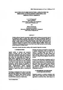
Figure 1a shows the interval fitting pattern of adjusted boxplot and proposed modification around the true 95% boundaries in χ2 distribution for small sample size. In graphical representation marker for different techniques are fixed as blue circle represents the true boundary at 95%, Maroon Square represent the fences constructed by ABP and dark grey triangles are fixed for MBP in all figures. It is observed that on the lower side, fence of MBP is close to true boundary for low level skewness. As the skewness increase performance of both techniques becomes equal as their fences overlap each other. For the upper side of the fence again looking at figure 1a for small sample size it can be seen that line of fence values of MBP is close to true fence and large gap can be seen between true upper boundary and ABP technique upper fence. As the sample size increases from small to medium sample, performance of ABP improved bit on lower side of the distribution. While comparing the fences on the upper side of the distribution the performance of proposed technique is significantly better than fence of ABP. Similarly figure1-c shows the fences for large sample size and performance of MBP on upper side of chi square distribution can be seen in comparison to ABP. Considering both sides at the same time that performance of ABP is bit better on lower side in medium and large sample sizes which is negligible. On upper side of the distribution performance of MBP is significantly better than ABP.

96



Figure 1:

Fences Comparison in Small, Medium and Large Sample Sizes: Chi Square Fig 1-a: Comparison of True 95% boundaries with ABP and MBP

0

20

40

60

Chi Square Small Sample Size

.5

1

1.5

2

skewness truelcv abplfs mbplfs

trueucv abpufs mbpufs

ABP Adjusted Boxplot: MBP Modified Boxplot

Fig1-b: Comparison of True 95% boundaries with ABP and MBP

0

10 20 30 40 50

Chi Square Medium Sample Size

.5

1

1.5

2

skewness truelcv abplfm mbplfm

trueucv abpufm mbpufm


Fig1-c: Comparison of True 95% boundaries with ABP and MBP

0

10 20 30 40 50

Chi Square Large Sample Size

.5

1

1.5

2

skewness truelcv abplfl mbplfl

trueucv abpufl mbpufl


NOTE: abplfs, abpufs, abplfm, abpufm, abplfl, abpufl, are the lower and upper fences for small, medium and large sample size in adjusted boxplot and modified boxplot respectively.


97


-0.35

-0.40

-0.49

-0.62

0.76

0.79

0.82

0.85

ABP LF

0.61

0.64

0.67

0.70

MBP LF

0.73

0.76

0.80

0.84

100

ABP LF

0.67

0.69

0.72

0.75

MBP LF

0.73

0.76

0.80

0.84

500

ABP LF

0.68

0.71

0.73

0.76

MBP LF

0.73

0.76

0.80

0.84

0.96

0.97

0.98

0.99

ABP UF

1.01

1.02

1.02

1.02

MBP UF

1.01

1.02

1.03

1.03

100

ABP UF

0.99

1.00

1.01

1.01

MBP UF

1.01

1.02

1.03

1.03

500

Table 2: Fences of ABP and MBP and True 95% Boundary in β Distribution Sample Size

Moment Measure of Skewness

ABP UF

0.98

0.99

1.00

1.01

MBP UF

1.01

1.02

1.03

1.03

25

True Lower Fence (2.5%)

25

True Upper Fence (97.5%)

Figure 2 shows the fence construction of ABP and MBP techniques around 95% true boundaries in β distribution. Since β is selected with parameters which are negatively skewed, so outliers on the upper tail (Compressed side of distribution) will be deficient while outliers on the lower tail (extended side of the distribution) will be excess outliers intuitively. Figure 2a shows that for the small sample size, on the upper tail fence values of ABP and MBP techniques overlap each other and have the same distance from the true upper boundary. By looking at the lower side of the distribution, it can be observed that true lower boundary and lower fence constructed by MBP are very close while the lower fence of ABP technique has a large gap from the true lower boundary. By increasing the sample size to medium and large, performance of ABP improved on the right side of the distribution as compared to MBP while on the lower side of the distribution performance of MBP is better. Overall it can be stated that there is tradeoff between both methodologies in medium and large sample sizes while performance of MBP is better in small sample size as compared to ABP. So on the basis of 95% true boundary it can be said that MBP is constructing fence close to the true 95% boundary in β distribution.

98



Figure 2: Fences Comparison in Small, Medium and Large Sample Sizes: Beta Fig2-a: Comparison of True 95% boundaries with ABP and MBP

.6

.7

.8

.9

1

Beta Small Sample Size

-.6

-.55

-.5 skewness truelcv abplfs mbplfs

-.45

-.4

-.35




.7

.8

.9

1

1.1

Beta Medium Sample Size

-.6

-.55

-.5 skewness truelcv abplfm mbplfm

-.45

-.4

-.35



Fig-2-c: Comparison of True 95% boundaries with ABP and MBP

.7

.8

.9

1

1.1

Beta Large Sample Size

-.6

-.55

-.5 skewness truelcv abplfl mbplfl

-.45

-.4

-.35





99


Table 3: Fences of ABP and MBP and True 95% Boundary in Lognormal Distribution Sample Size

Moment Measure of Skewness

0.61

1.32

2.26

3.69

6.18

0.68

0.46

0.31

0.21

0.14

ABP LF

0.44

0.12

-0.07

-0.19

-0.27

MBP LF

0.49

0.06

-0.27

-0.51

-0.66

ABP LF

0.55

0.28

0.11

0.00

-0.07

MBP LF

0.49

0.09

-0.15

-0.25

-0.27

ABP LF

0.57

0.31

0.15

0.04

-0.04

MBP LF

0.49

0.11

-0.08

-0.09

-0.08

1.48

2.19

3.24

4.80

7.10

ABP UF

1.98

3.64

6.37

10.67

17.21

MBP UF

1.58

2.32

3.41

5.11

7.78

ABP UF

1.78

3.11

5.28

8.66

13.69

MBP UF

1.57

2.33

3.54

5.64

9.12

ABP UF

1.73

2.98

5.01

8.17

12.89

MBP UF

1.57

2.34

3.66

6.20

10.32

500

100

25

True Lower Fence (2.5%)

500

100

25

True Upper Fence (97.5%)

Figure 3a shows the fences of ABP and MBP around the 95% true boundary in small sample size of the lognormal distribution. It can be observed that MBP is constructing fence accurately over the 95% true boundary for small sample size. For ABP it is obvious that on the lower tail it performs pretty well but on the upper tail its performance falls badly and fence of ABP is away from true 95% boundary. The gap of ABP fence from true upper boundary is large as level of skewness increases. Even for the large sample size (figure 3c) it can be seen that although the gap of MBP has increased on the right tail but it is still in midway of ABP technique and true boundary for the lower tail (compressed side of the distribution). Similar pattern can be observed for medium and large samples can be observed in figure 3b and 3c respectively.

100



Figure 3:

Fences Comparison in Small, Medium and Large Sample Sizes: Lognormal Fig3-a: Comparison of True 95% boundaries with ABP and MBP

0

5

10

15

20

Lognormal Small Sample Size

0

2

4

6

skewness truelcv abplfs mbplfs




0

5

10

15

Lognormal Medium Sample Size

0

2

4

6

skewness truelcv abplfm mbplfm



Fig3-c: Comparison of True 95% boundaries with ABP and MBP

0

5

10

15

Lognormal Large Sample Size

0

2

4

6

skewness truelcv abplfl mbplfl





101


8. Discussion and Conclusion It can be observed from the above tables/graphs that performance of ABP improves as the sample size increases. At some places it competes with the performance of proposed technique for large sample sizes but at some places performance of MBP is better even in large sample sizes. In chi square distribution performance of both techniques are same on left side of distribution (compressed side of distribution) while performance of MBP is better on the right side of the distribution (extended side). Similar situation can be observed in all distribution under consideration. One more thing that is possible to compare if on one side performance of ABP is better and on other side MBP is better. Then comparison is possible only by adding the absolute discrepancies of fences from the true lower and upper boundaries. It can also be judged from the fences constructed by both techniques that total discrepancy of MBP is less than total discrepancy of ABP. Adjusted box plot however works in large sample size but it fails badly to construct the fence around the true central 95 percent boundary of the distribution in small samples. In real life researchers often face the problem of short sample and especially in annual or five yearly data. Proposed modification constructs fence close to true boundary than the existing technique in all sample sizes. It resolves the problem of generating large fence which hide mild outliers and some time constructs displaced fence. So it can be concluded that the proposed technique is equally useful in both small and large data sets as compare to adjusted boxplot. References 1. 2. 3. 4. 5. 6. 7.

102

Carling, K. (2000). Resistant outlier rules and the non-Gaussian case. Computational Statistics and Data Analysis, 33, 249-258. G. Brys, M. H. (2004). A Robust Measure of Skewness. Journal of Computational and Graphical Statistics, 13 (4), 996-1017. Hair, J. F., Tatham, R. L., Anderson, R. E., & Black, W. (1998). Multivariate Data Analysis (5th ed.). Prentice Hall. Hubert, M., & Vandervieren, E. (2008). An Adjusted Boxplot for Skewed Distributions. Computational Statistics and Data Analysis, 52, 5186–5201. Iglewicz, B., & Hoaglin, D. C. (1993). How to Detect and Handle Outliers. 16, Wisconsin: ASQC Quality Press. Kimber, A. C. (1990). Exploratory Data Analysis for Possibly Censored Data From Skewed Distributions. Applied Statistics, 39 (1), 21-30. Tukey, J. W. (1977). Exploratory data analysis. Addison-Wesely.
