Using boundary layer equilibrium to reduce ... - Atmos. Chem. Phys
Recommend Documents
Sep 16, 2011 - m denote quantities at the free-troposphere level just above the mixed-layer and averaged within the mixed layer, respec- tively. The surface ...
Jul 13, 2009 - conditions, weak winds and/or strong low-level temperature inversion ... in the wind protected area near small river lake in the .... It is widely used Eulerian photo- chemical ...... photochemistry in alpine valleys, Atmos. Chem.
Dec 23, 2013 - Correspondence to: A. H. Berner ([email protected]). Received: 21 June 2013 â Published in Atmos. Chem. Phys. Discuss.: 8 July 2013.
Jan 25, 2010 - uration in a cloud parcel (Nenes and Seinfeld, 2003). Higher. CDNC leads to an enhanced cloud albedo (Twomey, 1991). This effect is known ...
Jan 21, 2016 - Investigations of boundary layer structure, cloud characteristics and vertical mixing of aerosols at Barbados with large eddy simulations.
Dec 23, 2013 - plored with extended two-dimensional (2-D) simulations of up to 20 days, mostly ... tions support the BakerâCharlson hypothesis of two distinct.
Sep 27, 2011 - Fig. 2. The average fields of (a) low cloud amount (%), (b) LWP (g mâ2), (c) Re (micron) derived from GOES-10 data during the flight time. (see ...
Dec 23, 2013 - domain. An initial 50 % aerosol reduction is applied to half of the model ...... check domain sensitivity, run W5/NA100/LD (not shown) repeated ...
Jul 18, 2017 - Gregory R. Wentworth4, Maurice Levasseur8, Ralf M. Staebler9, Sangeeta ...... phy, J. G., Murphy, B. N., Kodros, J. K., Abbatt, J. P., and. Pierce ...
Nov 20, 2015 - of dust storms in the Sahara and the eastern Mediterranean in April 2012. ... and China (Zhang et al., 2014; Sun et al., 2013). Aerosol particles ...
Apr 16, 2007 - by low biogenic production due to cold weather, phenolog- ical stage of the isoprene ..... 211 pptv and 28 pptv in the winter and summer, respectively. .... ever, they both conducted measurements in August when temperature ...
Jul 18, 2017 - the Creative Commons Attribution 3.0 License. Boundary layer ... (campaign mean of 116 ± 8pptv) compared to July 2014. (campaign mean of ...
Sep 27, 2011 - Observations of the boundary layer, cloud, and aerosol variability in the southeast Pacific near-coastal marine stratocumulus during. VOCALS- ...
Jul 18, 2011 - *now at: University of California, Los Angeles, Dept. of Atmospheric & Oceanic Sciences, Los ... power spectra and the integral length scale of cross-stream ..... and water vapor and wind speed sharply increase with height,.
Jun 21, 2006 - and peroxides) were measured by more than one tech- nique/group allowing intercomparisons to be made. Prior to this study little was known ...
Feb 8, 2006 - the proximity of housing to the research site the operation of ... surements by sonic anemometers at 7 m (yellow line), 10 m (red line), 15 m (black line) and 24 m (green line), ... The opposite occurred a few hours after dawn.
and spring periods of the year, which is in nice agreement. Atmos. Chem. Phys., 3 ..... to compare the autumn and spring period between Aspvreten and Värriö.
Wood, C. R., Lacser, A., Barlow, J., Padhra, A., Belcher, S., Nemitz,. E., Helfter, C., Famulari, D., and Grimmond, C. S. B.: Turbulent flow at 190m above London ...
Biraud, S. C., Torn, M. S., Smith, J. R., Sweeney, C., Riley, W. J., and Tans, P. P.: A ... 34.9. 136.8. Chubu Centrair International Airport, Japan. ITM. 34.8. 135.4.
âEstimates of global terrestrial isoprene emissions using MEGAN. (Model of Emissions of Gases and Aerosols from Nature)â published in Atmos. Chem. Phys., 6 ...
It provides further insights into the details of the activity data, estimations of ...... Re-charging, repair work and recovery is always done off site by specialist.
Mar 17, 2016 - ber 2004 to June 2006, of 67µgmâ3 which is higher than the WHO annual .... lated is multiplied by the coverage factor k = 2. The relative ...
blue, S1 posterior = red). The full site names and details are provided in Table 1. 1800. 1900. 2000. 2100. 2200. 2300. CH. 4. (ppb). CHL. 1800. 1900. 2000.
Using boundary layer equilibrium to reduce ... - Atmos. Chem. Phys
Sep 16, 2011 - Levy et al., 1999; Lloyd et al., 2001; Styles et al., 2002), and ...... Chatfield, C.: The Analysis of Time Series, Chapman & Hall, New. York, USA, p.
Using boundary layer equilibrium to reduce uncertainties in transport models and CO2 flux inversions I. N. Williams1 , W. J. Riley2 , M. S. Torn2 , J. A. Berry3 , and S. C. Biraud2 1 Department
of Geophysical Sciences, University of Chicago, Chicago, IL, USA Berkeley National Laboratory, Earth Sciences Division, Berkeley, CA, USA 3 Carnegie Institution of Washington, Stanford, CA, USA 2 Lawrence
Received: 18 February 2011 – Published in Atmos. Chem. Phys. Discuss.: 13 April 2011 Revised: 27 August 2011 – Accepted: 30 August 2011 – Published: 16 September 2011
Abstract. This paper reexamines evidence for systematic errors in atmospheric transport models, in terms of the diagnostics used to infer vertical mixing rates from models and observations. Different diagnostics support different conclusions about transport model errors that could imply either stronger or weaker northern terrestrial carbon sinks. Conventional mixing diagnostics are compared to analyzed vertical mixing rates using data from the US Southern Great Plains Atmospheric Radiation Measurement Climate Research Facility, the CarbonTracker data assimilation system based on Transport Model version 5 (TM5), and atmospheric reanalyses. The results demonstrate that diagnostics based on boundary layer depth and vertical concentration gradients do not always indicate the vertical mixing strength. Vertical mixing rates are anti-correlated with boundary layer depth at some sites, diminishing in summer when the boundary layer is deepest. Boundary layer equilibrium concepts predict an inverse proportionality between CO2 vertical gradients and vertical mixing strength, such that previously reported discrepancies between observations and models most likely reflect overestimated as opposed to underestimated vertical mixing. However, errors in seasonal concentration gradients can also result from errors in modeled surface fluxes. This study proposes using the timescale for approach to boundary layer equilibrium to diagnose vertical mixing independently of seasonal surface fluxes, with applications to observations and model simulations of CO2 or other conserved boundary layer tracers with surface sources and sinks. Results indicate that frequently cited discrepancies between observations and inverse estimates do not provide sufficient proof of systematic errors in atmospheric transport models. Some previously Correspondence to: I. N. Williams ([email protected])
hypothesized transport model biases, if found and corrected, could cause inverse estimates to further diverge from carbon inventory estimates of terrestrial sinks.
1
Introduction
Coupled carbon-climate models predict that the fraction of anthropogenic CO2 emissions absorbed by ecosystems will decline over the 21st century (Friedlingstein et al., 2006; Denman et al., 2007), but how accurately these models represent current ecosystem CO2 sources and sinks remains unclear. Uncertainties in ecosystem sources and sinks result from errors in atmospheric transport models used to infer ecosystem exchanges from concentration measurements (Denning et al., 1995; Dargaville et al., 2003; Baker et al., 2006). The strongest vertical mixing coincides with ecosystem uptake, in summer, with weaker vertical mixing in winter when ecosystems release CO2 . This covariance between atmospheric dynamics and ecosystem exchanges, known as the seasonal rectifier effect, produces enhanced annual-mean near-surface concentrations in northern latitudes even over annually-balanced ecosystems (Fung et al., 1983; Denning et al., 1995). Inversions of modeled transport having erroneously strong rectification will compensate by overestimating northern and underestimating tropical terrestrial sinks, to balance the global CO2 budget (Denning et al., 1995; Stephens et al., 2007). Observational constraints could help reconcile atmospheric inversions that infer strong northern terrestrial sinks, with carbon inventories that estimate weaker northern but stronger tropical terrestrial sinks. However, different observations support different conclusions about transport model errors that would imply either stronger or weaker northern
Published by Copernicus Publications on behalf of the European Geosciences Union.
9632
I. N. Williams et al.: Boundary layer equilibrium and CO2 inversions
terrestrial sinks. Boundary layer mixing intuitively plays a role in rectification of CO2 vertical gradients, by diluting the effects of summer northern terrestrial uptake through deeper mixing. Atmospheric transport models tend to underestimate summer mixing depths (Denning et al., 1995; Chen et al., 2004; Yi et al., 2004; Denning et al., 2008), but correcting these errors could lead to even larger inferred northern terrestrial sinks in the inversions (e.g. Denning et al., 1995; Yi et al., 2004), increasing the discrepancy with terrestrial carbon inventories. On the other hand, differences between modeled and observed CO2 vertical profiles suggest systematically overestimated summer vertical mixing (Stephens et al., 2007), implying that transport model inversions would support weaker northern and stronger tropical terrestrial sinks if other aspects of the models were improved, such as tropospheric transport and cloud mass fluxes. Comparisons of transport models and observations have not taken into account the timescale dependence of transport and mixing, which has led to hypotheses of both overestimated and underestimated vertical mixing in transport models, corresponding to both overestimated and underestimated northern terrestrial carbon sinks in the inversions. The dilution by transient boundary layer growth approximately balances surface CO2 fluxes when analyzed during the daytime or over a few days (Raupach, 1991; Raupach et al., 1992; Levy et al., 1999; Lloyd et al., 2001; Styles et al., 2002), and can successfully explain the diurnal rectifier effect (Yi et al., 2004). However over longer periods of time boundary layer depth reflects a statistical equilibrium between surface heat fluxes acting to increase, and radiative cooling acting to decrease boundary layer depth, with clouds coupled through their effect on radiative cooling (Betts et al., 2004). Radiative cooling in turn balances adiabatic warming in subsiding branches of the circulation, bringing boundary layer trace gas concentrations into a statistically steady state that reflects an approximate equilibrium between surface fluxes and transport by the subsiding flow (Helliker et al., 2004; Betts et al., 2004). This paper uses boundary-layer equilibrium concepts to interpret discrepancies between modeled and observed concentration gradients in terms of transport model errors. Our results show that these discrepancies most likely result from overestimated as opposed to underestimated vertical transport and mixing, implying overestimated northern terrestrial carbon sinks in the inversions. However we find that seasonal concentrations alone cannot distinguish transport model errors from errors in prior-specified surface fluxes, and propose a new diagnostic to isolate the effects of transport and mixing.
Atmos. Chem. Phys., 11, 9631–9641, 2011
2
Methods
2.1
Mixed-layer approximation
The tracer conservation equation allows us to relate transport and mixing to modeled or observed trace gas concentrations. We assume dry convection maintains well-mixed trace gases in the boundary layer, and refer to this boundary layer as the mixed-layer. The corresponding tracer conservation equation (e.g. Betts, 1992) is given by ρm
where h, cf , cm , ρ, w, v, and ∇ are the mixed-layer depth, free troposphere and mixed-layer trace gas mixing ratios, atmospheric molar density, vertical wind velocity evaluated at the mixed layer height, horizontal wind velocity vector, and horizontal gradient operator, respectively; subscripts f and m denote quantities at the free-troposphere level just above the mixed-layer and averaged within the mixed layer, respectively. The surface flux or net ecosystem exchange (F ) balances the sum of mixed-layer CO2 storage (first left-hand side term), entrainment of free-troposphere CO2 owing to growth of the mixed-layer into the free-troposphere (second term), vertical advective transport averaged over the mixedlayer (third term), and horizontal advection (fourth term). Note the horizontal gradient operator and horizontal wind vector have components in both the meridional and zonal directions, and therefore the horizontal advection term includes both meridional and zonal advection. It helps to keep in mind that the terms involving ∂h/∂t (first and second left-hand side terms of Eq. (1)) and the vertical advection (third left-hand side term) represent two separate physical processes (Betts, 1992). The former accounts for entrainment of free-troposphere CO2 by the mixed-layer growing into the free-troposphere, whereas the latter implicitly accounts for the entrainment of free-troposphere CO2 that has descended to the top of the mixed-layer through vertical CO2 advection. We refer to these processes as entrainment and vertical advective transport, respectively, but use the term vertical transport and mixing when referring to the combination of both processes. Note also that net loss of mixed-layer air to the free-troposphere by ascending winds does not directly affect mixed-layer concentrations, in which case we must replace cf with cm as the top boundary condition on CO2 in Eq. (1). This dynamic boundary condition arises because the mixed-layer top moves relative to the vertical wind, and vice versa. We computed the first and second left-hand side terms of Eq. (1) from day-to-day changes in afternoon (01:00–04:00 p.m. local time) mixed-layer depths and concentrations. Turbulence becomes shallow and surface emissions (e.g., ecosystem respiration) accumulate in a shallow nocturnal boundary layer at night. However the rapid decay of turbulence after sunset leaves a relic mixed-layer, or www.atmos-chem-phys.net/11/9631/2011/
I. N. Williams et al.: Boundary layer equilibrium and CO2 inversions so-called residual layer, extending from the nocturnal boundary layer to the depth of the afternoon mixed-layer, where CO2 concentrations are similar to the afternoon mixed-layer (Yi et al., 2001). Therefore, we take zf as the total depth of the residual-layer and mixed-layer system and integrate (Eq. 1) over the diurnal cycle by assuming (1) much larger depth-integrated advective tendencies (third and fourth terms of Eq. 1) in the residual layer than in the nocturnal boundary layer, due to the much larger residual layer depth and wind speed; and (2) steady nighttime vertical concentration gradients between free-troposphere and residual layer that can be approximated by afternoon concentrations. Any accumulation of CO2 in the shallow nocturnal boundary layer shows up in the mixed-layer concentrations the following day. Previous studies used these same approximations in various forms, to close the CO2 budget over diurnal cycles (Chou et al., 2002; Bakwin et al., 2004; Helliker et al., 2004; Yi et al., 2004).
3
Measurements and model data
Our study uses atmospheric concentration measurements collected at the Central Facility (36.61◦ N, 97.49◦ W) of the US Southern Great Plains Atmospheric Radiation Measurement Climate Research Facility (SGP) between January 2003 and January 2008. More than 80 % of the land surface of the Southern Great Plains is managed for agriculture and grazing (Fischer et al., 2007). Winter wheat grows from November through June over 40 % of the region (Fischer et al., 2007), mostly to the southeast (Riley et al., 2009), with the remaining area dominated by pasture (40 %) and a mixture of C3 and C4 crops (20 %) that grow from April through August (Cooley et al., 2005). A precision gas system (Bakwin et al., 1995) was used to obtain mixed-layer CO2 concentrations at 15-minute intervals on the 60 m tower. Pressurized air samples have been collected approximately weekly on the 60 m tower and in the free-troposphere at SGP for subsequent analysis at NOAA/ESRL. The continuous mixed-layer CO2 concentrations were compared with the flask-based measurements to account for and correct possible drifts. These flask-based measurements include, but are not limited to, CO2 , CH4 , CO, N2 O, CO, SF6 , H2 , and 13 C and 18 O in CO2 . The sample collection procedures have been described in detail in Conway et al. (1994). Typically, air was pumped into a pair of 2.5L glass flasks, connected in series, and slightly pressurized above ambient pressure. For the free-troposphere concentrations we used the first available flask sample just above the CT/TM5 mixed-layer depth (samples were typically available at altitudes of 457.2, 609.6, 914, 1219.2, 1524, 1828.8, 2133.6, 2438.4, and 2743.2 m above ground, and higher, with an uncertainty of about 30 m). The 2008 CarbonTracker data assimilation system (hereafter CT/TM5) provided mixed-layer depths and threewww.atmos-chem-phys.net/11/9631/2011/
9633
dimensional distributions of CO2 mole fractions and surface fluxes at 1◦ ×1◦ spatial resolution every 3-h (Peters et al., 2007). CT/TM5 accounts for the effect of surface energy forcing on mixed-layer depth, through the prognostic energy budget in the underlying transport model (Transport Model 5, Krol et al., 2005). CT/TM5 incorporates surface flux measurements and model representations of ecosystem exchanges in a global, two-way nested atmospheric transport model driven by meteorological fields from the European Centre for Medium-Range Weather Forecasts (ECMWF). Our analysis includes observations from the SGP tower, and CT/TM5 data averaged over the two model grid points nearest to three sites including SGP, described in the section above; LEF (45.95◦ N, 90.27◦ W), characterized by a managed forest of mixed northern hardwood, aspen, and wetlands; and Harvard Forest (HFM, 42.54◦ N, 72.17◦ W), a managed, deciduous forest. These sites correspond to some of the North American aircraft flask sampling locations used in a related study (Stephens et al., 2007). The CT/TM5 dataset did not archive vertical advection, which we recreated here with vertical velocities from the ECMWF interim reanalysis, based on the same general circulation model and parameterization schemes in CT/TM5. Differences between CT/TM5 and our recreated advective tendencies are expected in part due to differences in the forecast time-steps used to create each dataset, and interpolation of the ECMWF meteorological data from 1.5◦ ×1.5◦ to 1◦ ×1◦ resolution in CT/TM5. We averaged the two CT/TM5 grid-points closest to each of our study sites for use with the ECMWF reanalysis vertical velocities, due to the difference in resolution of these products. Additional spatial averaging had little effect on the results. Resolution sensitivity of the recreated vertical advective tendency was investigated by spatially averaging ECMWF velocities over the 1 through 4 grid-cells nearest the SGP site, and was found to be small. Sensitivity was further tested using vertical velocities from three independent data assimilation systems (RUC, NCEP, and NARR), which were qualitatively similar to ECMWF velocities and did not have a notable effect on our results.
4 4.1
Timescale dependence Scaling
Previous studies made approximations to the conservation equation (Eq. 1) by neglecting either entrainment and storage (Bakwin et al., 2004; Helliker et al., 2004) or vertical advection (e.g. Yi et al., 2004), referred to here as the equilibrium and non-equilibrium approximations, respectively. The choice of approximation has important implications for transport model errors. We apply dimensional analysis to Eq. (1) to inform the appropriate approximation, by scaling the ratio of the sum of CO2 storage and entrainment to vertical advection according to the ratio of a Atmos. Chem. Phys., 11, 9631–9641, 2011
9634
I. N. Williams et al.: Boundary layer equilibrium and CO2 inversions
mixed-layer relaxation time (τ ) to a characteristic timescale (T ) of Eq. (1). We introduce the mixed-layer relaxation time as the ratio of characteristic mixed-layer depth to a characteristic subsidence rate (τ = H /W ). We refer to the ratio of these timescales as t ∗ = H /W T . The timescale (T ) can be chosen to represent the timescale of interest, for the purpose of scaling the advective and storage and entrainment terms. Note that we later apply a running time-average to Eq. (1), which imposes a lower limit on the timescale T as determined by the averaging time. The relaxation time τ = H /W characterizes how long it takes for tracer concentrations to come into equilibrium with vertical transport by the subsiding flow. The characteristic subsidence rate W reflects the aggregate of all processes affecting subsidence, including synoptic systems. Frontal passages and other mechanisms of ascent are coupled to subsidence through the conservation of mass and energy (e.g. Lawrence and Salzmann, 2008). Adiabatic warming approximately balances infrared radiative cooling in the subsiding branches of the circulation, which in turn balances latent heating by moist convection in the precipitating storm systems that comprise the ascending branches. Dimensional analysis predicts that the equilibrium approximation applies to the seasonal cycle when the relaxation time is significantly shorter than a season (i.e. t ∗ 1), in which case the storage and entrainment terms can be neglected relative to vertical advection. We tested this prediction by calculating the storage, entrainment, and vertical advection in Eq. (1) and applying a running average for averaging times ranging from 1 to 90 days. The averaging time corresponds to the shortest timescale resolved by the averaged equation, which helps quantify the relative importance of each process at different timescales. We added storage and entrainment together to form a single budget term, and divided the timeseries of this and the other terms into nonoverlapping segments of length ranging from 1 to 90-days, to obtain a statistical ensemble of CO2 budgets for each averaging time. We used non-overlapping segments to minimize statistical dependence among ensemble members. The 90-day non-overlapping segments have only one sample for each season in each year, for a total of 5 and 7 ensemble members for the SGP and CT/TM5 data, respectively (one for each year of data), whereas the 45-day non-overlapping segments contain 10 and 14 ensemble members, and so on. We quantified the relative importance of each term as a function of timescale, by taking the magnitudes of these budget terms, and taking the ensemble-median of their ratios (Figs. 1 and 2). Our results imply that previous studies based on nonequilibrium approximations did not capture the transport and mixing processes most important at seasonal timescales, when surface fluxes (Fig. 1) and vertical advective transports (Fig. 2) exceed storage and entrainment by an order of magnitude. We obtained similar results when calculating the budget terms from observed concentrations at SGP Atmos. Chem. Phys., 11, 9631–9641, 2011
Fig. 1. Ratios of the sum of entrainment and storage to net surface flux, for various averaging times between 1 and 90-days during June, July, August (JJA) and December, January, and February (DJF). Ratios were calculated using the CT/TM5 model output at all three sites (SGP, LEF, HFM), combined with meteorological data from ECMWF (see text for details).
(Fig. 2a). The non-dimensional number t ∗ quantifies the relative decrease in net storage and entrainment with increasing timescale, and also describes differences in timescale dependence across measurement sites related to regional-scale differences in subsidence rates and mixed-layer depths (see supplement and Fig. S1). More generally, the equilibrium approximation to Eq. (1) should include horizontal advection when similar in magnitude to vertical advection and surface fluxes. We included horizontal advection in our study of the seasonal cycle, shown in the following section. 4.2
Seasonal surface flux and CO2 budget
The seasonally-averaged CO2 budget confirms the smaller contribution of storage and entrainment relative to vertical advection, and shows that horizontal advection is smaller than vertical advection but of the same order of magnitude. These results hold whether calculating budget terms from observed concentrations at SGP (Fig. 3) or from CT/TM5 data for SGP, LEF and HFM (Fig. 4). We split the seasonallyaveraged vertical advection term into a linear and non-linear part (i.e., w1c = w1c + w 0 1c0 ), for reasons that will become clear in Sect. 5. This Reynolds decomposition follows from writing the components of vertical advection in terms of 90-day averages and departures from these averages (e.g., w = w+w0 , 1c = 1c+1c0 , where primes denote departures from the 90-day average) and 1c denotes the 90-day averaged vertical concentration gradient (1c = cm − cf ). The www.atmos-chem-phys.net/11/9631/2011/
I. N. Williams et al.: Boundary layer equilibrium and CO2 inversions
9635 3
a
2
b
1 0 −1
Flux (µmol m−2 s−1)
−2 −3 3 2 1 0 −1 −2 −3 3 2 1 0
Fig. 2. As in Fig. 1 but for the ratio of the sum of entrainment and storage to vertical advection calculated from 60-m tower and aircraft observations at SGP (a) and from CT/TM5 at SGP, LEF, and HFM (b).
−1
Horizontal Advection Nonlinear Vertical Advection
−2 −3 2001
2002
2003
2004
Year
2005
Total Vertical Advection Storage+Entrainment 2006
2007
2008
Fig. 4. Contribution of mixed-layer budget terms to the net surface flux calculated from CT/TM5 assimilated concentrations at SGP (a), LEF (b), and HFM (c).
Fig. 3. Contribution of mixed-layer budget terms to the surface flux at SGP, calculated from 90-day running averages using 60-m tower and aircraft mixing ratios, and decomposed into horizontal advection (green), vertical advection (blue), storage plus entrainment (red) and the sum of all terms (thick black).
non-linear vertical advection is on the order of the horizontal advection at SGP and LEF, which highlights the importance of weather disturbances on seasonal transport. The surface flux predicted using the equilibrium approximation (Fig. 5a, calculated from Eq. (1) after neglecting storage and entrainment terms) approximately agrees with the surface flux predicted from the data assimilation scheme internal to CT/TM5 (Fig. 5b). 5
Vertical gradients and rectifier effect
We explored the consequences of boundary layer equilibrium for vertical concentration gradients and the vertical rectifier effect, by using Eq. (1) and inverting the slowly-varying (seasonal) component of vertical advective transport, to predict the vertical concentration gradient (1c = cm − cf ), 1c = −(F + ρf w0 1c0 − ρm hv · ∇cm )/(ρf w)
(2)
where the second right-hand side term is the contribution of non-linear vertical advection (as defined in Sect. 4.2), the www.atmos-chem-phys.net/11/9631/2011/
last term is the contribution of vertically-integrated horizontal advection, and we have used the equilibrium approximation (neglecting storage and entrainment). Equation (2) illustrates why biases in seasonally-averaged vertical concentration gradients do not necessarily reflect systematic errors in modeled transport or mixing, since 1c is also affected by possible systematic errors in the seasonal surface flux (F ). These results confirm the importance of vertical and horizontal advective transports in determining the vertical distribution of CO2 in the lower troposphere. The equilibrium approximation (Eq. 2) successfully predicts the seasonal cycle and differences in vertical concentration gradients between the three sites. The equilibrium vertical gradients (Fig. 6a) compare favorably with those predicted by CT/TM5 (Fig. 6b) at all three sites (SGP, LEF, HFM), although we see differences in the seasonal cycle magnitude in some years. We did not compare panels (Fig. 6a and b) directly because differences between CT/TM5 and the equilibrium approximation were within the sensitivity of our results to increasing or decreasing the mixed-layer depth by one model level. We explored how seasonality in vertical transport contributes to seasonal rectification, by examining height-time cross sections of the vertical wind field (Fig. 7, top three panels), with seasonal variability in mixed-layer depth overlaid as solid black lines in the top three panels of Fig. 7. The cross section shows the 90-day running average subsidence velocities as a function of height above the surface, for the seven annual timeseries extending from 1 January–31 December, for January 2001–2008. Note that the 90-day average subsidence velocity at the 90-day average mixed layer depth (as indicated by the top three panels of Fig. 7) is not Atmos. Chem. Phys., 11, 9631–9641, 2011
9636
I. N. Williams et al.: Boundary layer equilibrium and CO2 inversions
Surface Flux (µmol m−2 s−1)
(a) 2 0 −2
(b) 2 0 −2 2001
2002
2003
SGP
2004 2005 Year
2006
LEF
2007
2008
rates vary seasonally, so that both contribute to the rectifier effect. In fact we find an anti-correlation between mixedlayer depths and subsidence rates at HFM, where the coincidence of strongest subsidence with strongest respiratory fluxes in winter helps to reduce winter mixed-layer concentrations relative to the free troposphere, bringing the winter vertical gradients at HFM closer to those of other sites. Other locations across eastern North America and the eastern Atlantic also have reversed seasonality in subsidence rates (see Supplement, Fig. S2), possibly related to topographic forcing and stationary wave patterns (Saltzman and Irsch, 1972).
HFM
Fig. 5. Surface flux inferred from the equilibrium approximation (a) and the CT/TM5 assimilated surface flux (b) for SGP (red), LEF (dashed black), and HFM (blue), using 90-day averages. Equilibrium fluxes (a) are given by the sum of horizontal and total vertical advection shown in Fig. 4.
6
Relaxation times and vertical mixing diagnostic
Our results call for a new vertical mixing diagnostic that takes into account both the strength of the divergent circulation and mixed layer depth variations. The boundary layer relaxation time τ = H /W (see Sect. 4.1) provides one such measure, which we can estimate from autocorrelations of vertical concentration gradient fluctuations. To obtain the relationship between vertical mixing and concentration autocorrelations, we draw an analogy between Eq. (1) and a first-order autoregressive process defined by dX(t) + aX(t) = Z(t) dt
(3)
where X(t) is a continuous random variable, a is a constant, and Z(t) represents a white noise process with zero mean (e.g. Jones, 1975; Chatfield, 2004). We make this analogy explicit by rearranging Eq. (1) to yield
Fig. 6. Vertical mixing ratio gradient inferred from the equilibrium approximation (a) and from the CT/TM5 data assimilation system (b) at SGP (red), LEF (dashed black), and HFM (blue), using 90day averages.
exactly the same as the 90-day average of daily subsidence velocity calculated at daily mixed layer depths (shown in the bottom three panels of Fig. 7 in solid black lines), but the differences are small. Vertical velocity increases monotonically with height in the lowest 1–2 km, since vertical velocity must vanish at the earth’s surface in the absence of topography. The results show that mixed layer depth alone does not fully explain the seasonal rectification of vertical concentration gradients. Subsidence rates vary seasonally and therefore also contribute to the seasonal rectifier effect (contours in top panels of Fig. 7). We see the expected increase in vertical mixing in summer, which results primarily from increased mixing depths at SGP and LEF (cf. solid and dashed lines in the lower three panels of Fig. 7). Deeper mixed layers can engage in stronger mass exchanges with the freetroposphere, because subsidence rates typically increase with height. However both mixed-layer depth and subsidence Atmos. Chem. Phys., 11, 9631–9641, 2011
d (h1c) + h∇ · vih1c = G(t) dt
(4)
where we assumed that free-troposphere mixing ratios vary slowly in time compared to mixed layer mixing ratios. Note that h1c is analogous to X(t) in Eq. (3) and the equation is evaluated at a fixed latitude and longitude. We used the vertically-integrated continuity equation, ρf w = −ρm h∇ · vih
(5)
to relate the subsidence rate at the mixed-layer top (w in Eq. (1)) to the vertically-averaged horizontal wind divergence (bracketed term in Eq. (4)), assuming constant divergence in the mixed-layer and zero vertical velocity at the surface (e.g. Betts, 1992). The term G(t) represents the combination of surface fluxes and horizontal advection G(t) = F /ρm − hv · ∇cm .
(6)
The weighting of the vertical gradient (1c) by h in Eq. (4) reflects the fact that the divergent circulation transports more mixed-layer mass per surface area as the depth of the mixedlayer increases, requiring either larger surface flux or smaller tracer vertical gradients to balance tracer transport.
www.atmos-chem-phys.net/11/9631/2011/
I. N. Williams et al.: Boundary layer equilibrium and CO2 inversions
−1.25
−1
−0.5 −0.25
−0.5 −0.25
9637
−2 −1−0.75 −0.5
Fig. 7. Top: Mean annual cycle of subsidence velocity (where w < 0) calculated from ECMWF data (years 2001-2007), contoured every 0.25 cm s−1 , overlaid with CT/TM5 90-day running average maximum daily mixed layer height (error bars indicate standard deviation of the mean). Below: Subsidence velocity at the 90-day running average mixed layer top (wzf ) (solid line) and at the annual average (constant) mixed layer depth (dashed line). SGP (Summer)
∆ C Autocorrelation
1
SGP (Winter)
a
b
0.5
0 0
2
4
6
0 2 8 Time Lag (days)
4
6
8
Fig. 8. Autocorrelation coefficient for perturbations in daily vertical mixing ratio gradients from aircraft and 60-m tower observations (blue square markers), and from CT/TM5 (red circle markers). Error bars indicate the standard deviation of the mean over all years (2003–2005 for observations, 2001–2007 for CT/TM5). Panels (a) and (b) correspond to summer and winter, respectively. The gray line indicates exponential decay toward the 90-day average value, according to Eq. (7) (width of the line indicates the standard deviation).
The diagnostic follows from Eq. (4) after noting that the autocorrelation of a first-order autoregressive process decays exponentially as a function of time lag, with a rate constant a (cf. Eq. (3)). We therefore expect the autocorrelation of perturbations in h1c to decay according to A = exp[−h∇ · vi(t − t 0 )]
www.atmos-chem-phys.net/11/9631/2011/
(7)
where A is the autocorrelation function, and t − t 0 is the time lag of the autocorrelation (e.g. Chatfield, 2004). We apply this Eq. (7) to perturbations in h1c about the seasonal average (i.e. h1c − h1c) so that G(t) has zero seasonal mean, by analogy to Z(t). Note that this perturbation form of Eq. (4) is derived by subtracting the seasonal average of Eq. (4) from both sides of the same equation. We compared observed (blue markers in Fig. 8) and theoretical autocorrelations for summer (June, July, August), and winter (December, January, February) respectively, where we used 60-m tower and aircraft flask samples to calculate autocorrelations of observed vertical gradients at SGP. The gray lines in Fig. (8) indicate the theoretical estimate from ECMWF reanalysis horizontal wind divergence using Eq. (7). Sensitivity tests revealed that weighting the vertical gradients by h (as in Eq. (4)) had little effect on the autocorrelations, so we show autocorrelations of the vertical concentration gradients (1c) alone, for simplicity. A comparison of CT/TM5 (red markers in Fig. 8) to observed autocorrelations (blue markers in Fig. 8) reveals no major differences in diagnosed divergence rates at SGP. We estimated divergence rates of 6.23×10⁻⁶ and 1.04×10⁻⁵ s−1 for summer and winter, respectively, by a non-linear leastsquares fit of Eq. (7) to the CT/TM5 autocorrelations. We obtained similar divergence rates from the observed autocorrelations (6.10×10⁻⁶ and 1.13×10⁻⁵ s−1 for summer and winter, respectively), which correspond to subsidence velocities of about 1 and 0.7 cm s−1 , for typical mixed-layer depths, in approximate agreement with reanalysis estimates (cf. Fig. 7). Differences in sample means between the Atmos. Chem. Phys., 11, 9631–9641, 2011
I. N. Williams et al.: Boundary layer equilibrium and CO2 inversions
Height
9638
FreeTroposphere Mixed Layer
Mixing Ratio
Fig. 9. Panel (a): Schematic illustrating a hypothetical perfect summer transport model simulation (solid circles) forced with either summer overestimated continental mixed-layer concentrations or overestimated prior surface flux, and the observed free-troposphere and mixed layer concentrations (squares). Panel (b): as in (a) but for a hypothetical transport model simulation having correctly specified prior surface fluxes but overestimated vertical mixing. Panel (c): as in (b) but for underestimated vertical mixing. The mixed layer is indicated in gray shading.
CT/TM5 and observationally-derived divergence rates (e.g. between 6.23×10⁻⁶ for CT/TM5 and 6.10×10⁻⁶ s−1 for observations, in summer) were not statistically significant, and would amount to vertical concentration gradient errors on the order of 0.1 ppm (using 1c ∼ −F w−1 from Eq. (2)), much smaller than the errors reported in a previous study at other sites (Stephens et al., 2007). These results do not necessarily conflict with previous work suggesting large errors in vertical transport and mixing (Stephens et al., 2007), particularly because we have not applied our diagnostic to sites showing large discrepancies between observations and transport models inversions. The CT/TM5 vertical concentration gradient is inconsistent with ECMWF reanalysis subsidence rates at HFM (see supplement, Fig. S2), which warrants further study, but those subsidence rates are model-derived and so may also be in error. Note that CT/TM5 comes into closer agreement with carbon inventories and has overall smaller concentration profile errors compared to the TransCom3 model inversions (Peters et al., 2007). Also, CT/TM5 uses a higher resolution (two-way nested) version of the TM5 model than what inverse studies have used, and assimilates observed and modelderived surface fluxes every 3-h, including effects of interannual variability and vegetation fires. Our proposed diagnostic has the capability of determining if the systematic errors seen in transport model inversions result from errors in the modeled divergent wind field. Transport model inversions predict vertical concentration gradients almost twice as large as observations at some sites (Stephens et al., 2007). The equilibrium boundary layer approximation implies that these errors should appear as similarly large errors in mixed-layer divergence rates, or equivalently in subsidence rates at the mixed-layer depth (i.e. twice as fast in transport models as in observations, according to 1c ∼ −F w−1 ). Such large errors are on the order of the difference between winter and summer divergence rates at SGP, which is statistically significant in our analysis, and therefore should be detectable using the methods presented here.
Atmos. Chem. Phys., 11, 9631–9641, 2011
We conclude that boundary layer relaxation times can diagnose vertical transport and mixing relevant to seasonal CO2 budgets. Drawbacks to this method include the requirement that fluctuations about the seasonally averaged surface flux represent temporally uncorrelated noise. The validity of this assumption will vary according to the measurement site, but could be tested by comparing autocorrelations of CO2 to those of other conserved tracers whose surface fluxes are less likely to be correlated at sub-seasonal timescales. Previous studies reported mixed-layer SF6 autocorrelations (Denning et al., 1999), which were similar to our results using CO2 , but were not compared to the divergent wind field. Our work provides a method to relate these concentration statistics to transport and mixing in atmospheric models. 7
Discussion
Boundary layer equilibrium has important consequences for the interpretation of CO2 flux inversion errors. Given the surface flux, equilibrium predicts a simple inverse proportionality between CO2 vertical gradients and the vertical wind (1c ≈ −F w−1 ), consistent with the hypothesis that models systematically underestimate summer vertical gradients due to overestimated vertical mixing (Stephens et al., 2007). However, the simple inverse proportionality between errors in vertical gradients and mixing only works when there are no systematic errors in the surface flux, horizontal advective transport, or non-linear vertical advective transport (i.e., synoptic-scale eddies), according to Eq. (2). Systematic biases in vertical gradients could also result from errors in the initial fluxes specified in Bayesiansynthesis inversions, or in the biospheric models used for these inversions (and in CT/TM5), without having to invoke systematic transport model errors. Other studies also suggested inversion errors due to these prior fluxes, possibly resulting from seasonality in fossil fuel emissions (Gurney et al., 2005; Erickson et al., 2008) or errors in the seasonal amplitude or timing of modeled biospheric fluxes (Peters www.atmos-chem-phys.net/11/9631/2011/
I. N. Williams et al.: Boundary layer equilibrium and CO2 inversions et al., 2007; Yang et al., 2007), which were not considered in past analyses of inversion sensitivity. Previous studies using SF6 did not indicate such large systematic errors in summer modeled transport (Gloor et al., 2007; Patra et al., 2009). Overestimated prior fluxes would overestimate boundarylayer CO2 concentrations relative to the free-troposphere in forward transport model simulations (Fig. 9a), similar to observed errors (Stephens et al., 2007) in transport model inversions. As a counter example to the hypothesis that vertical mixing is systematically biased in transport models, consider a hypothetical transport model simulation having perfect vertical mixing and transport but subject to specification of overestimated summer prior surface fluxes (shown schematically in Fig. 9). Accurate transport implies that subsidence (w < 0) in this simulation always matches that of the real atmosphere. Overestimated summer fluxes (i.e. F less negative than observed) require larger free-tropospheric concentrations in the forward simulation (solid circles in Fig. 9a) than in observations (squares in Fig. 9a), and correspondingly weaker vertical gradients, according to 1c ≈ −F w−1 . Unless the inversion of this transport is tightly constrained to observed concentrations, the post-inversion vertical gradient may remain underestimated, falsely indicating summer overestimated mixing, while free-tropospheric concentrations would remain overestimated, falsely indicating underestimated summer mixing. This example illustrates why either CO2 concentrations or vertical CO2 gradients taken alone do not always indicate transport model errors, and how opposite conclusions about these errors can be drawn when free-troposphere concentrations are considered separately of mixed-layer concentrations. Previous studies cited underestimated model mixed layer depths as a mechanism for underestimated summer mixing (Yi et al., 2004; Denning et al., 2008), and as an explanation for underestimated seasonal amplitudes of modeled freetropospheric and column-average CO2 (Yang et al., 2007). However, we found an anticorrelation between mixed-layer depth and the strength of the divergent circulation at some sites, such that vertical mixing diminishes in summer when the boundary layer is deepest. We illustrate these errors schematically in Fig. 9b,c (circles and squares indicate model and observations, respectively). Boundary layer equilibrium predicts that underestimated summer mixing should lead to overestimated vertical concentration gradients (Fig. 9c), whereas observational studies found underestimated gradients (Stephens et al., 2007). In the case of overestimated summer mixing (Fig. 9b), the hypothetical perfect prior flux would be adjusted to take up more CO2 in order to minimize differences between the forward-transport simulation and observations, after the inversion procedure. Overestimated summer mixing would therefore be more desirable with regard to explaining why the northern land carbon sink is stronger in inversion estimates than in land carbon inventories. www.atmos-chem-phys.net/11/9631/2011/
9639
The equilibrium boundary layer approach does not consider mixing by convective clouds, and so may underestimate the extent to which spring and summer flux inversions could be in error due to transport model errors. However, the resolved-scale subsidence velocity in the data assimilation systems used here accounts for the larger-scale effects of transport and mixing at the sub-grid scale, due to separate enforcement of mass and energy balance at both subgrid and global scales in the models underlying these datasets (Lawrence and Salzmann, 2008). This process is reflected in the reasonable agreement between surface fluxes and vertical gradients from data assimilation systems and those reconstructed using the equilibrium approximation and resolvedscale model winds. Improvements to the parameterization of mixing and transport by convective clouds are still needed, especially since these parameterizations were designed to realistically simulate energy balances for climate studies rather than tracer transport. 8
Conclusions
Previously reported discrepancies between modeled and observed concentration gradients most likely result from overestimated as opposed to underestimated vertical transport and mixing, implying overestimated northern terrestrial carbon sinks in the inversions. However, seasonal concentration gradients alone cannot distinguish between transport model errors and errors in prior-specified surface fluxes, according to boundary layer equilibrium concepts. We propose using the additional information contained in concentration gradient fluctuations, to diagnose vertical mixing errors independently of errors in seasonal surface fluxes. Previous studies assumed that boundary layer depth indicates vertical mixing strength, whereas we found anticorrelations between these quantities at some sites. Underestimated model boundary layer depth therefore does not provide sufficient evidence to conclude that transport models underestimate northern terrestrial sinks. Vertical CO2 advection by the divergent wind field strongly contributes to observed vertical concentration gradients, and does not always track boundary layer depth. We recommend considering subsidence or mass divergence rates together with boundary layer depth when assessing transport model errors. The equilibrium approximation neglects much of the complexity of atmospheric transport and mixing, yet even this simplified description contains more degrees of freedom than typical diagnostics constrain. Our results imply that discrepancies between modeled and observed vertical concentration profiles alone are not sufficient to prove that the models have systematic vertical transport and mixing errors. The methods developed here provide additional observational constraints needed to diagnose the several factors leading to errors and uncertainties in transport model inversions.
Atmos. Chem. Phys., 11, 9631–9641, 2011
9640
I. N. Williams et al.: Boundary layer equilibrium and CO2 inversions
Supplementary material related to this article is available online at: http://www.atmos-chem-phys.net/11/9631/2011/ acp-11-9631-2011-supplement.pdf. Acknowledgement. Funding for this study was provided by the US Department of Energy, BER Program, Contract # DEAC02-05CH11231. CarbonTracker 2008 results provided by NOAA ESRL, Boulder, Colorado, USA from the website at http://carbontracker.noaa.gov. Andy Jacobson assisted with the CarbonTracker data. Edited by: C. Gerbig
References Baker, D. F., Law, R. M., Gurney, K. R., Rayner, P., Peylin, P., Denning, A. S., Bousquet, P., Bruhwiler, L., Chen, Y. H., Ciais, P., Fung, I. Y., Heimann, M., John, J., Maki, T., Maksyutov, S., Masarie, K., Prather, M., Pak, B., Taguchi, S., and Zhu, Z.: TransCom 3 inversion intercomparison: Impact of transport model errors on the interannual variability of regional CO2 fluxes, 1988-2003, Global Biogeochem. Cy., 20, GB1002, doi:10.1029/2004GB002439, 2006. Bakwin, P. S., Tans, P. P., Zhao, C. L., Ussler, W., and Quesnell, E.: Measurements of carbon-dioxide on a very tall tower, Tellus B – Chem. Phys. Meteorol., 47, 535–549, 1995. Bakwin, P. S., Davis, K. J., Yi, C., Wofsy, S. C., Munger, J. W., Haszpra, L., and Barcza, Z.: Regional carbon dioxide fluxes from mixing ratio data, Tellus B – Chem. Phys. Meteorol., 56, 301– 311, 2004. Betts, A. K.: FIFE Atmospheric boundary-layer budget methods, J. Geophys. Res.-Atmos., 97, 18523–18531, 1992. Betts, A. K., Helliker, B. R., and Berry, J. A.: Coupling between CO2 , water vapor, temperature, and radon and their fluxes in an idealized equilibrium boundary layer over land, J. Geophys. Res.-Atmos., 109, D18103, doi:10.1029/2003JD004420, 2004. Chatfield, C.: The Analysis of Time Series, Chapman & Hall, New York, USA, p. 50, 2004. Chen, B. Z., Chen, J. M., Liu, J., Chan, D., Higuchi, K., and Shashkov, A.: A Vertical Diffusion Scheme to estimate the atmospheric rectifier effect, J. Geophys. Res.-Atmos., 109, D04306, doi:10.1029/2003JD003925, 2004. Chou, W. W., Wofsy, S. C., Harriss, R. C., Lin, J. C., Gerbig, C., and Sachse, G. W.: Net fluxes of CO2 in Amazonia derived from aircraft observations, J. Geophys. Res.-Atmos., 107(D22), 4614, doi:10.1029/2001JD001295, 2002. Conway, T. J., Tans, P. P., Waterman, L. S., and Thoning, K. W.: Evidence for interannual variability of the carbon-cycle from the National Oceanic and Atmospheric Administration Climate Monitoring and Diagnostics Laboratory Global Air-Sampling Network, J. Geophys. Res.-Atmos., 99, 22831–22855, 1994. Cooley, H. S., Riley, W. J., Torn, M. S., and He, Y.: Impact of agricultural practice on regional climate in a coupled land surface mesoscale model, J. Geophys. Res.-Atmos., 110, D03113, doi:10.1029/2004jd005160, 2005. Dargaville, R. J., Doney, S. C., and Fung, I. Y.: Inter-annual variability in the interhemispheric atmospheric CO2 gradient: con-
Atmos. Chem. Phys., 11, 9631–9641, 2011
tributions from transport and the seasonal rectifier, Tellus B – Chem. Phys. Meteorol., 55, 711–722, 2003. Denman, K., Brasseur, G., Chidthaisong, A., Ciais, P., Cox, P., Dickinson, R., Hauglustaine, D., Heinze, C., Holland, E., Jacob, D., Lohmann, U., Ramachandran, S., da Silva Dias, P., S.C., W., and Zhang, X.: Contribution of Working Group I to the Fourth Assessment Report of the Intergovernmental Panel on Climate Change, in: Climate Change 2007: The Physical Science Basis, edited by: Solomon, S., Qin, D., Manning, M., Chen, Z., Marquis, M., Averyt, K., Tignor, M., and Miller, H., Cambridge University Press, Cambridge, UK and New York, NY, USA, 2007. Denning, A. S., Fung, I. Y., and Randall, D.: Latitudinal gradient of atmospheric CO2 due to seasonal exchange with land biota, Nature, 376, 240–243, 1995. Denning, A. S., Holzer, M., Gurney, K. R., Heimann, M., Law, R. M., Rayner, P. J., Fung, I. Y., Fan, S. M., Taguchi, S., Friedlingstein, P., Balkanski, Y., Taylor, J., Maiss, M., and Levin, I.: Three-dimensional transport and concentration of SF6 - A model intercomparison study (TransCom 2), Tellus Series B – Chem. Phys. Meteorol., 51, 266–297, 1999. Denning, A. S., Zhang, N., Yi, C. X., Branson, M., Davis, K., Kleist, J., and Bakwin, P.: Evaluation of modeled atmospheric boundary layer depth at the WLEF tower, Agr. For. Meteorol., 148, 206–215, 2008. Erickson, D. J., Mills, R. T., Gregg, J., Blasing, T. J., Hoffman, F. M., Andres, R. J., Devries, M., Zhu, Z., and Kawa, S. R.: An estimate of monthly global emissions of anthropogenic CO2 : Impact on the seasonal cycle of atmospheric CO2 , J. Geophys. Res.Biogeosci., 113, G01023, doi:10.1029/2007jg000435, 2008. Fischer, M. L., Billesbach, D. P., Berry, J. A., Riley, W. J., and Torn, M. S.: Spatiotemporal variations in growing season exchanges of CO2 , H2 O, and sensible heat in agricultural fields of the Southern Great Plains, Earth Interact., 11, 1–21, 2007. Friedlingstein, P., Cox, P., Betts, R., Bopp, L., Von Bloh, W., Brovkin, V., Cadule, P., Doney, S., Eby, M., Fung, I., Bala, G., John, J., Jones, C., Joos, F., Kato, T., Kawamiya, M., Knorr, W., Lindsay, K., Matthews, H. D., Raddatz, T., Rayner, P., Reick, C., Roeckner, E., Schnitzler, K. G., Schnur, R., Strassmann, K., Weaver, A. J., Yoshikawa, C., and Zeng, N.: Climate-carbon cycle feedback analysis: Results from the (CMIP)-M-4 model intercomparison, J. Climate, 19, 3337–3353, 2006. Fung, I., Prentice, K., Matthews, E., Lerner, J., and Russell, G.: 3dimensional tracer model study of atmospheric CO2 – Response to seasonal exchanges with the terrestrial biosphere, J. Geophys. Res.-Ocean. Atmos., 88, 1281–1294, 1983. Gloor, M., Dlugokencky, E., Brenninkmeijer, C., Horowitz, L., Hurst, D. F., Dutton, G., Crevoisier, C., Machida, T., and Tans, P.: Three-dimensional SF6 data and tropospheric transport simulations: Signals, modeling accuracy, and implications for inverse modeling, J. Geophys. Res.-Atmos., 112, D15112, doi:10.1029/2006JD007973, 2007. Gurney, K. R., Chen, Y. H., Maki, T., Kawa, S. R., Andrews, A., and Zhu, Z. X.: Sensitivity of atmospheric CO2 inversions to seasonal and interannual variations in fossil fuel emissions, J. Geophys. Res.-Atmos., 110, D10308, doi:10.1029/2004JD005373, 2005. Helliker, B. R., Berry, J. A., Betts, A. K., Bakwin, P. S., Davis, K. J., Denning, A. S., Ehleringer, J. R., Miller, J. B., Butler, M. P., and Ricciuto, D. M.: Estimates of net CO2 flux by application
www.atmos-chem-phys.net/11/9631/2011/
I. N. Williams et al.: Boundary layer equilibrium and CO2 inversions of equilibrium boundary layer concepts to CO2 and water vapor measurements from a tall tower, J. Geophys. Res.-Atmos., 109, D20106, doi:10.1029/2004JD004532, 2004. Jones, R. H.: Estimating the variance of time averages, J. Appl. Meteorol., 14, 159–163, 1975. Krol, M., Houweling, S., Bregman, B., van den Broek, M., Segers, A., van Velthoven, P., Peters, W., Dentener, F., and Bergamaschi, P.: The two-way nested global chemistry-transport zoom model TM5: algorithm and applications, Atmos. Chem. Phys., 5, 417– 432, doi:10.5194/acp-5-417-2005, 2005. Lawrence, M. G. and Salzmann, M.: On interpreting studies of tracer transport by deep cumulus convection and its effects on atmospheric chemistry, Atmos. Chem. Phys., 8, 6037–6050, doi:10.5194/acp-8-6037-2008, 2008. Levy, P. E., Grelle, A., Lindroth, A., Molder, M., Jarvis, P. G., Kruijt, B., and Moncrieff, J. B.: Regional-scale CO2 fluxes over central Sweden by a boundary layer budget method, Agr. For. Meteorol., 98-9, 169–180, 1999. Lloyd, J., Francey, R. J., Mollicone, D., Raupach, M. R., Sogachev, A., Arneth, A., Byers, J. N., Kelliher, F. M., Rebmann, C., Valentini, R., Wong, S. C., Bauer, G., and Schulze, E. D.: Vertical profiles, boundary layer budgets, and regional flux estimates for CO2 and its C-13/C-12 ratio and for water vapor above a forest/bog mosaic in central Siberia, Global Biogeochem. Cy., 15, 267–284, 2001. Patra, P. K., Takigawa, M., Dutton, G. S., Uhse, K., Ishijima, K., Lintner, B. R., Miyazaki, K., and Elkins, J. W.: Transport mechanisms for synoptic, seasonal and interannual SF6 variations and ”age” of air in troposphere, Atmos. Chem. Phys., 9, 1209–1225, doi:10.5194/acp-9-1209-2009, 2009. Peters, W., Jacobson, A. R., Sweeney, C., Andrews, A. E., Conway, T. J., Masarie, K., Miller, J. B., Bruhwiler, L. M. P., Petron, G., Hirsch, A. I., Worthy, D. E. J., van der Werf, G. R., Randerson, J. T., Wennberg, P. O., Krol, M. C., and Tans, P. P.: An atmospheric perspective on North American carbon dioxide exchange: CarbonTracker, Proc. Natl. Acad. Sci. USA, 104, 18925–18930, 2007. Raupach, M. R.: Vegetation-atmosphere interaction in homogeneous and heterogeneous terrain - some implications of mixedlayer dynamics, Vegetatio, 91, 105–120, 1991.
www.atmos-chem-phys.net/11/9631/2011/
9641
Raupach, M. R., Denmead, O. T., and Dunin, F. X.: Challenges in linking atmospheric CO2 concentrations to fluxes at local and regional scales, Austr. J. Bot., 40, 697–716, 1992. Riley, W. J., Biraud, S. C., Torn, M. S., Fischer, M. L., Billesbach, D. P., and Berry, J. A.: Regional CO2 and latent heat surface fluxes in the Southern Great Plains: Measurements, modeling, and scaling, J. Geophys. Res.-Biogeosci., 114, G04009, doi:10.1029/2009JG001003, 2009. Saltzman, B. and Irsch, F. E.: Note on the theory of topographically forced planetary waves in atmosphere, Mon. Weather Rev., 100, 441–444, 1972. Stephens, B. B., Gurney, K. R., Tans, P. P., Sweeney, C., Peters, W., Bruhwiler, L., Ciais, P., Ramonet, M., Bousquet, P., Nakazawa, T., Aoki, S., Machida, T., Inoue, G., Vinnichenko, N., Lloyd, J., Jordan, A., Heimann, M., Shibistova, O., Langenfelds, R. L., Steele, L. P., Francey, R. J., and Denning, A. S.: Weak northern and strong tropical land carbon uptake from vertical profiles of atmospheric CO2 , Science, 316, 1732–1735, 2007. Styles, J. M., Lloyd, J., Zolotoukhine, D., Lawton, K. A., Tchebakova, N., Francey, R. J., Arneth, A., Salamakho, D., Kolle, O., and Schulze, E. D.: Estimates of regional surface carbon dioxide exchange and carbon and oxygen isotope discrimination during photosynthesis from concentration profiles in the atmospheric boundary layer, Tellus B – Chem. Phys. Meteorol., 54, 768–783, 2002. Yang, Z., Washenfelder, R. A., Keppel-Aleks, G., Krakauer, N. Y., Randerson, J. T., Tans, P. P., Sweeney, C., and Wennberg, P. O.: New constraints on Northern Hemisphere growing season net flux, Geophys. Res. Lett., 34, L12807, doi:10.1029/2007GL029742, 2007. Yi, C., Davis, K. J., Bakwin, P. S., Denning, A. S., Zhang, N., Desai, A., Lin, J. C., and Gerbig, C.: Observed covariance between ecosystem carbon exchange and atmospheric boundary layer dynamics at a site in northern Wisconsin, J. Geophys. Res.-Atmos., 109, D08302, doi:10.1029/2003JD004164, 2004. Yi, C. X., Davis, K. J., Berger, B. W., and Bakwin, P. S.: Longterm observations of the dynamics of the continental planetary boundary layer, J. Atmos. Sci., 58, 1288–1299, 2001.