USING BOX-SCORES TO DETERMINE A ...

USING BOX-SCORES TO DETERMINE A POSITION’S CONTRIBUTION TO WINNING BASKETBALL GAMES

by Garritt L. Page

A Project submitted to the faculty of Brigham Young University in partial fulfillment of the requirements for the degree of

Master of Science

Department of Statistics Brigham Young University August 2005

BRIGHAM YOUNG UNIVERSITY

GRADUATE COMMITTEE APPROVAL

of a Project submitted by Garritt L. Page

This Project has been read by each member of the following graduate committee and by majority vote has been found to be satisfactory.

Date

Dr. Gilbert W. Fellingham, Chair

Date

Dr. C. Shane Reese

Date

Dr. Bruce J. Collings

BRIGHAM YOUNG UNIVERSITY

As chair of the candidate’s graduate committee, I have read the Project of Garritt L. Page in its final form and have found that (1) its format, citations, and bibliographical style are consistent and acceptable and fulfill university and department style requirements; (2) its illustrative materials including figures, tables, and charts are in place; and (3) the final manuscript is satisfactory to the graduate committee and is ready for submission to the university library.

Date

Dr. Gilbert W. Fellingham Chair, Graduate Committee

Accepted for the Department

G. Bruce Schaalje Graduate Coordinator

Accepted for the College

G. Rex Bryce Associate Dean, College of Physical and Mathematical Sciences

ABSTRACT

USING BOX-SCORES TO DETERMINE A POSITION’S CONTRIBUTION TO WINNING BASKETBALL GAMES

Garritt L. Page Department of Statistics Master of Science

Basketball is a sport that has become increasingly popular world-wide. At the professional level it is a game in which each of the five positions has a specific responsibility that requires unique skills. It seems likely that it would be valuable for coaches to know which skills for each position are most conducive to winning. Knowing which skills to develop for each position could help coaches optimize each player’s ability by customizing practice to contain drills that develop the most important skills for each position that would in turn improve the teams overall ability. Through the use of Bayesian hierarchical modeling and NBA boxscore performance categories, this project will determine how each position needs to perform in order for their team to be successful.

Acknowledgements

I would like to thank Dr. Fellingham and Dr. Reese for their guidance and suggestions that ultimately made this project a successful learning experience. Also I would like to thank all those who participated in countless brainstorming discussions from which many good ideas were generated. Finally I would like to thank Elizabeth, my wife, who bravely endured the Provo experience.

Contents

Chapter

1 Introduction

1

2 Literature Review

5

2.1

Bayesian Statistics . . . . . . . . . . . . . . . . . . . . . . . . . . .

2.2

Sports Statistics . . . . . . . . . . . . . . . . . . . . . . . . . . . . . 11

2.3

5

2.2.1

Bayesian Methods Applied to Sports Data . . . . . . . . . . 11

2.2.2

Studies on the Sport of Basketball . . . . . . . . . . . . . . . 13

2.2.3

General Sports Papers . . . . . . . . . . . . . . . . . . . . . 15

Bayesian Regression

. . . . . . . . . . . . . . . . . . . . . . . . . . 16

3 The Model

18

3.1

Data . . . . . . . . . . . . . . . . . . . . . . . . . . . . . . . . . . . 18

3.2

Model . . . . . . . . . . . . . . . . . . . . . . . . . . . . . . . . . . 20 3.2.1

The Hierarchical Model . . . . . . . . . . . . . . . . . . . . . 20

3.2.2

The Likelihood . . . . . . . . . . . . . . . . . . . . . . . . . 22

3.2.3

Prior Distributions . . . . . . . . . . . . . . . . . . . . . . . 23

xi

3.3

Computation . . . . . . . . . . . . . . . . . . . . . . . . . . . . . . 28

3.4

Convergence Diagnostics . . . . . . . . . . . . . . . . . . . . . . . . 29

3.5

Model Checking . . . . . . . . . . . . . . . . . . . . . . . . . . . . . 29

4 Results

30

4.1

Convergence and Cross Validation . . . . . . . . . . . . . . . . . . . 30

4.2

Positional Summaries . . . . . . . . . . . . . . . . . . . . . . . . . . 37

4.3

Simulation . . . . . . . . . . . . . . . . . . . . . . . . . . . . . . . . 41

5 Further Research and Potential Model Improvements

44

5.1

Bench Players . . . . . . . . . . . . . . . . . . . . . . . . . . . . . . 44

5.2

Interaction Terms . . . . . . . . . . . . . . . . . . . . . . . . . . . . 45

5.3

Likelihood and Data Concerns . . . . . . . . . . . . . . . . . . . . . 46

5.4

Conclusions . . . . . . . . . . . . . . . . . . . . . . . . . . . . . . . 46

Appendix

A Code Appendix

48

A.1 FORTRAN code . . . . . . . . . . . . . . . . . . . . . . . . . . . . 48 A.2 R code . . . . . . . . . . . . . . . . . . . . . . . . . . . . . . . . . . 65 A.3 SAS code . . . . . . . . . . . . . . . . . . . . . . . . . . . . . . . . 80

B Gibbsit Function Output

C Time Series Plots

90

105

xii

Bibliography

108

xiii

xiv

Tables

Table 1.1

Typical NBA Box-Score . . . . . . . . . . . . . . . . . . . . . . . .

3

3.1

Hyperparameter Values . . . . . . . . . . . . . . . . . . . . . . . . . 28

4.1

Cross Validation Results . . . . . . . . . . . . . . . . . . . . . . . . 32

4.2

Percent of correct cross validation predictions . . . . . . . . . . . . 34

4.3

Posterior means, standard deviations, and 95% highest posterior density credible intervals of parameters of assists, steals, turnovers, free throws made, free throw percentage for each position . . . . . . 37

4.4

Posterior means, standard deviations, and 95% highest posterior density credible intervals of parameters for field goals made, field goal percentage, offensive rebounds, and defensive rebounds for each of the positions . . . . . . . . . . . . . . . . . . . . . . . . . . . . . 38

xv

xvi

Figures

Figure 4.1

Plots of the posterior predictive distribution for game 1116 of the cross validation data. The first five players are members of the New York Knicks the last four are members of the Indiana Pacers. The vertical line represents the difference in score which is -3 for New York and 3 for Indiana which is what we tried to predict. . . . . . . 33

4.2

Plots of posterior distributions of parameters for assists, steals, turn overs, offensive rebounds, and defensive rebounds for each position . 35

4.3

Plots of posterior distributions of parameters for free throws made, free throw percentage,field goals made, and field goal percentage for each position . . . . . . . . . . . . . . . . . . . . . . . . . . . . . . 36

4.4

Plots of the posterior distributions of nine selected parameters using the generated data. The mean of the parameter from generated data is represented by the vertical line . . . . . . . . . . . . . . . . 43

C.1 Time series plots for selected µβh,j ’s . . . . . . . . . . . . . . . . . . 106 xvii

C.2 Time series plots for selected variance, team, game, and regression coefficient parameters . . . . . . . . . . . . . . . . . . . . . . . . . . 107

xviii

Chapter 1

Introduction

Basketball is a sport that has become increasingly popular world-wide. At the professional level it is a game in which each of the five positions has a specific responsibility that requires unique skills. In order for a team to be successful the team members should recognize their roles and combine them so as to play as a single unit (Bray and Brawley 2002). It seems likely that it would be valuable for coaches to know which skills for each position are most conducive to winning. Knowing which skills to develop for each position could help coaches optimize each player’s ability by customizing practice to contain drills that develop the most important skills for each position, which would in turn improve the team’s overall ability. The purpose of this project is to determine which skills a particular basketball player needs at his position to help his team be successful. For example, under certain offensive systems, a point guard’s main objective would be to direct the team’s offense, which often requires good passing and ball handling skills. A coach could then include drills to develop the skills relevant to being a point guard.

1

It seems reasonable that some abilities have varying importance according to position. For example, a turnover from a guard could possibly be more detrimental to the outcome of the game than a turnover from the center position. A turnover from a guard can occur on the perimeter, which leads to a fast break opportunity for the opposing team. A turnover from a center generally occurs near the basket where the offense can make the transition to defense faster. Also, it seems plausible that defensive rebounds from the center position are more important to the outcome of the game than a defensive rebound from the shooting guard. If a center allows the opposition an offensive rebound it usually leads to an easy basket attempt, whereas a guard allowing an offensive rebound usually results in resetting the offense, which gives the defense time to reestablish itself. Each coach has a different style of play or coaching philosophy which can affect a player’s contribution. For example, Larry Brown of the Detroit Pistons is vocal about his dislike of point guards that try to score more often than pass. Under Coach Brown’s system a high scoring point guard is not desirable. The relative abilities of the other players on the team also should be considered. A team with a dominant center may not need as much point production from other positions. The results of NBA games are summarized in a box-score (see Table 1.1). In these box-scores the final score of the game, where the game was played, and each player’s totals for thirteen performance categories are given. These thirteen categories are field goals made, field goal attempts, free throws made, free

2

throw attempts, offensive rebounds, defensive rebounds, total rebounds, assists, personal fouls, steals, turnovers, and points. Through USA Today’s web site, http://www.usatoday.com/, we were able to obtain box scores for approximately 18,000 NBA regular season games from the 1996-1997 season to the 2003-2004 season. LA LAKERS (78) AT UTAH (104) LA LAKERS POS MIN == === F 24 F 35 C 24 G 19 G 41 23 17 15 10 12 17 3 240

FGM === 1 3 3 0 9 0 1 1 0 1 0 1 20

FGA === 8 10 8 2 21 3 5 2 1 3 4 1 68

FTM === 2 8 0 2 16 1 1 0 1 0 0 2 33

FTA === 2 10 2 2 20 2 2 0 2 0 0 2 44

OFF === 1 2 2 0 1 1 0 1 1 1 3 0 13

REBOUNDS DEF TOT === === 2 3 7 9 3 5 1 1 3 4 2 3 2 2 1 2 1 2 0 1 0 3 2 2 24 7

AST === 0 1 0 1 1 2 0 1 0 0 0 1 7

PF == 2 5 4 3 5 0 4 4 3 1 0 1 32

ST == 0 1 0 0 1 0 0 0 0 0 2 0 4

TO == 0 3 3 2 2 0 0 0 2 0 1 1 14

PTS === 4 14 6 2 38 1 3 2 1 3 0 4 78

PLAYER POS MIN ====== == === A KIRILENKO F 38 C BOOZER F 34 J COLLINS C 10 K MCLEOD G 29 G GIRICEK G 12 M OKUR 20 R BELL 25 M HARPRING 28 H EISLEY 19 C BORCHARDT 14 K SNYDER 9 K HUMPHRIES 2 TOTALS 240

FGM === 5 10 0 2 4 0 4 9 2 2 0 0 38

FGA === 6 13 1 7 9 4 8 11 7 3 3 3 75

FTM === 6 7 0 2 3 2 2 3 0 1 0 0 26

FTA === 7 10 0 2 3 2 2 3 0 2 0 0 31

OFF === 2 5 0 0 0 1 0 2 0 1 0 0 11

REBOUNDS DEF TOT === === 4 6 6 11 1 1 0 0 1 1 4 5 3 3 5 7 0 0 5 6 3 3 0 0 32 43

AST === 1 3 0 8 0 4 0 4 3 1 0 0 24

PF == 2 1 4 5 4 1 5 4 1 2 2 0 31

ST == 1 0 0 1 0 1 0 1 0 0 0 0 4

TO == 5 0 0 1 2 0 1 2 0 1 0 0 12

PTS === 16 27 0 6 11 2 10 23 4 5 0 0 104

PLAYER ====== C BUTLER L ODOM C MIHM C ATKINS K BRYANT T BROWN B COOK J JONES B GRANT L WALTON K RUSH S VUJACIC TOTALS UTAH

Table 1.1: Typical NBA Box-Score

In these box-scores only the players that started had their position identified. Therefore, our analysis will be constrained to include only players that started the game. In addition, these box-scores make no distinction between a point guard and a shooting guard or between a small forward and a power forward. Since point guards and shooting guards usually have vastly different roles within the framework of the team we wanted to be able to distinguish between 3

the two. So based on our personal recollection and using the internet as a further resource we separate the guards into point guards and shooting guards and the forwards into small forwards and power forwards. We will approach this problem from a hierarchical Bayesian point of view and will model the difference in the points scored, by the two competing teams, as a function of the difference of nine performance categories found in the box-score.

4

Chapter 2

Literature Review

The following literature review can be divided into three sections. The first section is a general review of Bayesian methods. The second is a review of papers written in a sports statistics framework. The third is a review of Bayesian regression models.

2.1

Bayesian Statistics

The Reverend Thomas Bayes is generally given credit for discovering Bayes’ Theorem because of a paper that was published after his death (Bayes 1764). The theorem, for two simple events A and B, states: P (B|A) =

P (A|B)P (B) . P (A)

(2.1)

Stigler (1983) addresses the issue that Bayes might have erroneously been given credit for first discovering the theorem. Hartley (1749) reveals that a friend of his found a solution for the inverse probability problem (that is, inverting the conditionality in probability). Hartley then provides Bayes’ Theorem and an explanation of the importance of the discovery. Since Hartley’s book was published 5

12 years before Thomas Bayes’ death, Stigler concludes that it is likely that Bayes was not the first person who discovered the theorem that carries his name. Bayes’ paper still gives a good example of the use of Bayes’ Theorem to estimate an unknown parameter. The transition from using simple events A and B to estimating parameters using Bayes’ Theorem is done by simply substituting a vector of parameters θ for B and a vector of data y for A. Therefore, for parameter estimation Bayes’ Theorem becomes:

π(θ|y) =

f (y|θ)π(θ) f (y)

=R

f (y|θ)π(θ) , f (y|θ)π(θ) d θ

(2.2) (2.3)

where π(θ|y) is called the posterior distribution of the parameters given the data, f (y|θ) is the likelihood (sometimes referred to as the sampling density or the distribution of the data given the parameters), π(θ) is the prior distribution of the parameters, and f (y) is the marginal density of the data. The denominators from equation (2.2) and (2.3) are equal by the law of total probability and are often referred to as the normalizing constant. Bayes constructed a binomial sampling density with an unknown probability of success (θ). He first estimated θ by rolling a ball on a billiard table and recording its horizontal coordinate, constrained to be between 0 and 1. He argued that a priori each horizontal coordinate is just as likely to be the resting place for the ball. Then a second ball was rolled n times and a success occured if the ball came to rest to the left of the first ball thrown. The random variable X was the

6

number of successes. Thus the sampling density of X would be

n p

θp (1 − θ)n−p .

Bayes was ultimately interested in finding the probability of θ being between two values given p successes. Since P (a < θ < b ∩ X = p) = P (X = p) =

Ra b

n p

θp (1 − θ)n−p dθ and

R 1 n 0

p

θp (1 − θ)n−p dθ, we can use Bayes’ Theorem to show: R a n p θ (1 − θ)n−p dθ b p P (a < θ < b|X = p) = R 1 n . p (1 − θ)n−p dθ θ 0 p

Here Bayes assumed a uniform distribution for θ so π(θ) = 1. He justified the analogy and uniform assumption in a scholium to his 1764 paper. (For a complete discussion on Bayes’ analogy and details on his probability propositions and controversies surrounding his 9th scholium see Stigler (1982) and Schafer (1982).) Laplace independently discovered Bayes’ Theorem in the late 18th century (Stigler 1986). He applied Bayes’ Theorem to estimate parameters in a binomial and hypergeometric setting. He assumed the probability of success in the binomial setting to be uniform, similar to Bayes, but did not give any justification for the assumption. In the hypergeometric case, he assumed that sampling from one of two possible urns, say A and B, is equally likely and then showed that Bayes’ Theorem gives the correct result. Even though Bayes’ Theorem was discovered in the 18th Century, as a modeling technique it was not widely used until the late 20th Century because of the difficulty of implementing even basic models. Consider the case of modeling a phenomena with a normal likelihood where the mean and variance are unknown and are given a normal and an inverse gamma as prior distributions. Even in this simple case obtaining the normalizing constant requires evaluating the non-trivial 7

integral found in the denominator of equation(2.3). Because of the difficulty of implementation, Bayesian methods were not practical for most of the 20th Century. The impracticality of Bayesian methods was remedied in the mid 20th Century unbeknownst to statisticians. Metropolis et al. (1953) created an algorithm implementing Markov Chain Monte Carlo (MCMC) and an acceptance/rejection rule that would generate draws from a target distribution under certain conditions. The first step is to choose a starting point for the parameter vector which will be noted as θ0 . The choice of starting value is not particularly important so long as the selection is not extremely strange (for example, choosing a negative value as the starting value for a variance parameter.) The second step is to draw a candidate parameter vector θcand from some symmetric distribution, where a symmetric distribution is on in which f (θa |θb ) = f (θb |θa ) for all θa and θb . Then the ratio of the densities, g(θcand |y) r= g(θt−1 |y)

(2.4)

is calculated, where g(·) is the numerator from equation(2.3) and is often referred to as the un-normalized posterior distribution. Finally, set cand with probability min(r, 1) θ t θ = t−1 θ otherwise. Then repeat the algorithm beginning with the second step. Hastings (1970) was able to generalize Metropolis’ algorithm by relaxing the requirement that the distribution from which θcand is drawn has to be symmetric.

8

The ratio r then becomes

r=

g(θcand |y)/p(θcand |θt−1 ) . g(θt−1 |y)/p(θt−1 |θcand )

(2.5)

This method of posterior estimation is known as the Metropolis-Hastings algorithm. Geman and Geman (1984) developed a special case of the MetropolisHastings algorithm called Gibbs sampling (see Gelman et al. 2004, chap. 11), which is useful in many multidimensional statistical models. In this algorithm the complete conditionals (i.e. conditional distributions) are used. They are defined as: [θj ] = (θj |θ1 , . . . , θj−1 , θj+1 , . . . , θk ).

(2.6)

Thus the complete conditional for θj is the value of θj conditioned on the other k parameters in the model. The Gibbs sampler can be implemented if a complete conditional is in the form of a distribution from which values can be easily drawn. If this is the case then the algorithm cycles through all of the complete conditionals in one iteration, therefore there are k steps for each iteration. Each complete conditional is updated on the latest values of the other complete conditionals which are at iteration t if they have already been updated, otherwise they are at iteration t-1. Inference using iteratively simulated draws, like MCMC, requires some diagnostic checks to insure convergence to the target distribution. Kass et al. (1998) ˆ which talk about different ways to check for convergence. They discuss the use of R

9

is the “. . . estimated posterior variance of the parameter, based on the mixture of all the simulated sequences, divided by the average of the variances with in each sequence.” They suggest running different chains by using different starting points ˆ is close to 1 for all parameters. until R Two other areas of concern are the number of iterations needed to fully explore the target distribution, and which iterates within the initial transient stage, often referred to as the burn, should be discarded. Raftery and Lewis (1992) determine the burn length and how many iterations are needed in order to estimate a quantile of the posterior distribution within some pre-specified range and a probability that the quantile lies in the pre-specified range. They implement this strategy in their gibbsit software, in which they give the necessary iterations and burn to obtain a desired posterior quantile and a probability that it is within a desired range. With the advance of computational methods, Bayesian methods are becoming more widely used and application to more complicated models is possible. Hierarchical models, which often estimate large numbers of parameters, are a natural progression in Bayesian analysis. These types of models allow us to estimate more parameters than there are data points. If the parameters come from the same population we can combine information for parameter estimation and “borrow strength” from the other parameters that follow the same distribution. Reese et al. (2001) implement a hierarchical model to estimate the fetal growth and gestation time for bowhead whales of the Bering, Chukchi, and Beaufort Seas

10

(BCBS) stock. They estimate the length of a fetus at birth, the growth rate, and the conception date for each whale. Solving this problem necessitated estimating 3n + 2 parameters with only n data points, which is possible using a Bayesian hierarchical model. They then model the fetal age as a function of growth rate, conception date and length of fetus at birth.

2.2

Sports Statistics

The following is a brief review of some methods that have been used to answer questions relating to sports. The first three papers use a Bayesian approach, the next three papers involve the sport of basketball, and the final papers are general sports papers.

2.2.1

Bayesian Methods Applied to Sports Data Berry et al. (1999) propose a method to characterize players’ talents regard-

less of era for baseball, golf, and hockey. This is difficult to do because players’ abilities are confounded with era, competition, and improvements in equipment among other things. They construct a logit additive Bayesian hierarchical model with a parameter for players ability, age, and era. Through these parameters they are able to bridge players from different eras by career overlap, take into account the competition of a particular era, and model the deterioration of skills due to aging. They use 1996 as a “benchmark” year. All evaluations of players are relative to this season. To estimate a league-wide age effect they compare each

11

player’s actual performance as they age to their estimated ability. The difficulty of a particular season is estimated by comparing a player’s performance in the season with their estimated ability and estimated age effect. They found that golf players have the most longevity and skill deteriorates the most rapidly in hockey players. Bayesian hierarchical methods are also used by Graves et al. (2003) to model permutations. The permutation of interest was the order in which auto racing drivers finish a race. First they estimate a driver’s ability where θij is the ith drivers ability in the j th race. Then a finishing order is determined by choosing a driver to finish in last place with a probability proportional to λij = exp(−θij ). Then a second-to-last-place finisher is chosen from the remaining drivers with probability proportional to exp(−θij ). This process is repeated until only two drivers remain, from which a second-place finisher is chosen with probability

λi1j . (λi1j +λi2j )

This produces an “attrition model”, from which they are able

to construct a likelihood. The model closely resembles what actually happens in auto-racing, that is, drivers often drop out one by one. With this model they are able to estimate a driver’s racing ability, calculate the probability of a driver winning from the current standing in which the driver is at, estimate how a driver’s ability varies from track to track, and predict which drivers will be successful in the future. In golf, deciding between a 3 iron or a 7 iron for a tee shot on a par 3 hole of length 200 yards with a green that is surrounded by water is usually made

12

based on past performance, current conditions, and intuition. Zellner (1999) uses a Bayesian analysis on this interesting golf problem. He assigns probabilities for the number of strokes needed to complete the hole for each club, and argues that using uniform probabilities or long run frequency would be inadequate in this situation. Rather, an appropriate utility function tailored to each score is used to choose the club for which the expected score is lower.

2.2.2

Studies on the Sport of Basketball A topic of debate in many sports is the notion of a “hot hand.” This is

claimed to occur when a player performs significantly above his average for an extended number of plays. Tversky and Gilovich (1989) address this topic for the sport of basketball. They argue that if a hot hand exists then there would be correlation within a sequence of shots. That is, making one shot would increase the chance of making the next shot. They perform an experiment by recording foul shots of some university athletes to get an estimate of the correlation between shots. They find that making a basket is largely independent of the outcome of the previous shot attempted. Bishop and Gajewski (2004) entertain the idea of being able to determine if a college player would be a success in the NBA. They use principal components, logistic regression, and cross validation to predict a players draftability. Each potential draft pick is rated by their physical size and the quality of their basketball skills. The rank of a player’s ability is derived from factors similar to those found

13

in a box-score. To reduce the number of variables, they use principle components to identify linear combinations that best explain the variance in the data and use these values to obtain a physical size ranking and an ability ranking. Then they use logistic regression and cross validation to predict a player’s draftability. They are successful in some predictions. For example, during the 2000-2001 season Jason Gardner from Arizona was selected as an All-American, but they predicted that he would not be a very successful player in the NBA, and in fact he was never drafted. Every March the National Collegiate Athletic Association (NCAA) Men’s Division I Basketball Tournament is held to determine the national champion. Teams are assigned a number 1 through 16 according to their ability within each of four regions. These numbers are referred to as seeds. 1 seeds are paired with 16 seeds, 2 seeds are paired with 15 seeds, and so forth. Since the tournament’s current format was implemented no 16-seed has beaten a 1-seed. Stern (1998) tries to determine if a 16-seed will ever beat a 1-seed in the NCAA Men’s Division I Basketball Tournament. He uses the point spread as a reasonable measure to estimate the difference in the abilities of the two teams. The difference between the actual game outcome and the point spread is found to roughly follow a Gaussian distribution. So the difference in score can be thought of as normal random variables with mean equal to the point spread and the standard deviation equal to 11. To estimate the probability of an i-seed defeating a j-seed, a logistic regression model is used to estimate the probability as a function of the difference in seeding.

14

He finds that a 16 seed will eventually defeat a 1-seed if the NCAA continues with its present format. In fact there is a 1 in 100 chance of it eventually happening.

2.2.3

General Sports Papers Berry (2001) talks about the amateur drafts for the four major sports

leagues: the National Football League (NFL), Major League Baseball (MLB), National Basketball Association (NBA), and National Hockey League (NHL). He is interested to see which of these four leagues does the better job in evaluating talent. To do this, a player selection is defined as a success if the player is eventually chosen as an all star. Berry models the log of the odds of a player becoming an all star as a function of the draft position. He finds that the NBA and NFL’s early draft picks are more likely to become all stars and that later draft picks have a better chance of becoming an all star in the NHL and MLB. Also for the NHL and MLB, Berry incorporates the positions of the players drafted and finds that there is little difference between positions. The quarterback ranking in the NFL is a confusing and often an inappropriate way to rate quarterbacks. White and Berry (2002) propose an alternative method to rate quarterbacks. The NFL’s method does not take into account the circumstances of the game when quantifying the importance of an action. White and Berry determine how important an action is in the context of the game by assigning an expected point count to each play and fitting a tiered logistic regression model. To obtain rankings they find the value of each play and then average

15

the point value over all plays for each quarterback. Randall Cunningaham of the Minnesota Vikings was the number one rated quarterback; this matched the NFL’s quarterback rating. One big difference between the rankings is illustrated by Rob Johnson of the Buffalo Bills. The NFL rank him as the second best quarterback in 1998, where as White and Berry rank him as 22nd out of 44 quarterbacks.

2.3

Bayesian Regression

Regression in general uses the conditional distribution of a response variable given an explanatory variable to make predictions and inference. It is one of the most widely used statistical tools. It assumes that the data have been drawn from a relation of the form: y = Xβ + where y is the response variable, X is a matrix of known explanatory variables, β is a vector of parameters to be estimated and is a random vector of independent identically distributed error terms. Gelman et al. (2004) dedicate chapters 14 and 15 of their book to regression models in a Bayesian framework. They say that a key difference between a Bayesian linear model and that of a frequentist perspective is setting up prior distributions on the model parameters that reflect substantive knowledge but are not so strong as to dominate the data inappropriately. Chen and Deely (1996) use a constrained Bayesian multiple regression model to predict the size of the upcoming apple crop in New Zealand. Their explanatory variable is the tree’s age, which they divide into ten different intervals, and the response variable is number of cartons of apples produced. The

16

youngest trees are associated with β1 and the oldest trees are associated with β10 . Since farmers usually don’t allow poor producing trees to live they constrain the parameters of interest so that 0 ≤ β1 ≤ β2 ≤ · · · ≤ β10 . That is, the older the tree the more apples it will produce. They choose a normal likelihood and assign a normal distribution for the β’s and an inverse gamma for σ 2 . They use the Gibbs sampler algorithm to perform MCMC, then fit the same model using ordinary least squares (OLS). They use the posterior predictive distribution to predict the upcoming apple crop using the Bayesian model and also predict the next apple crop using OLS.. They find that all of the parameters estimated using Bayesian methods preserve the constrained parameter space, whereas a few of the parameters estimated violated this space using OLS analysis. Smith (1973) examines the Bayesian hierarchical linear model. He shows that the Bayes estimates of the parameters in question have the structure of a weighted average between the least squares estimates and the prior mean.

17

Chapter 3

The Model

This chapter gives an overview of the model we will use. The chapter starts with a discussion on the data. The next section discusses the motivation behind the model, and then the hierarchical aspect of the model. Next the likelihood and prior distribution assignments are described. Then computation details, convergence checks, and model fit are examined.

3.1

Data

The box-score of the NBA is a table that displays 13 summary statistics for all players that enter a NBA game (see table 1.1). In the present study we focus on nine categories. They are: assists (ast), steals (stl), turnovers (tno), free throws made (ftm), free throw percentage (ftp), field goals made (fgm), field goal percentage (fgp), offensive rebounds (orb), and defensive rebounds (drb). The four categories that are not considered are minutes, total rebounds, fouls, and points. Minutes, although not explicitly in the model, are used to standardized the variables, which will be explained later in the paper. Total rebounds is a

18

linear combination of offensive rebounds and defensive rebounds and total points is a near linear combination of field goals made and free throws made, so including them in the model introduces collinearity. In the 1996-1997 season the NBA had 29 teams so we have T = 29 teams and O = 29 opponents. Each team has twelve players who can participate in the game but in this study we only focus on starters that play at least 45 games so we have P l = 131 players. We make the cut off 45 games because to make the playoffs a team needs to usually win around 45 games. Each of the five starters is assigned a position at the beginning of a game and we assume that he plays that position throughout the game, so we have P o = 5 positions and they are: point guard (pg), shooting guard (sg), small forward (sf), power forward (pf), and center (c). Because we are only including those players that have started at least 45 games there will be some teams for which some positions will not be represented. There are box-scores for 1163 games from the 1996-1997 season so we have G = 1163 games. All categories are standardized by minutes. That is, the player’s totals are divided by the total number of minutes played. Each player is paired by position (i.e. point guards from competing teams are paired and shooting guards from competing teams are paired, etc.) for each game and the differences for the nine standardized box-score categories between the matched players are computed. These differences become the explanatory variables. We use differences so that we might consider the talent level of the opposition. For example, a team whose

19

power forward scores 10 points and his opponent scores 5 points would probably be better off than a team whose power forward scores 25 points but his opponent scores 30. For the response variable we use the difference in the final score of the game. So players on the same team will always have the same observed response value for a given contest.

3.2

Model

We are interested in determining how players in each of the five positions need to perform in nine box-score categories so their team wins the game. We will use multiple regression to estimate the effect that each of these categories will have on the difference in the score of a basketball game. The regression model is: y = β0 +β1 ast+β2 stl+β3 tno+β4 f tm+β5 f tp+β6 f gm+β7 f gp+β8 orb+β9 drb (3.1) where y is the difference in the final score for a basketball game, β0 is the overall intercept, β1 is the effect that difference in assists (ast) has on the difference of the final score, β2 is the effect for difference in steals (stl), β3 the effect for the difference in turnovers (tno), etc.

3.2.1

The Hierarchical Model An inadequacy in equation (3.1) is the assumption that each β is the same

regardless of player or position. In addition, an assumption of independent identically distributed responses would be violated. The way in which the data are used creates dependence in the response variable for individuals on the same team, 20

the opponent they play, and the game in which they play. We obtain a separate β estimate for each player and deal with the dependency issues by incorporating a Bayesian hierarchical model on the regression coefficients and adding an effect for the team of which the player is a member, the opponent the player’s team is playing, and the game in which they are competing. Thus the model becomes yiklm = γm + τk + φl + β1i ast + β2i stl + β3i tno + β4i f tm + β5i f tp+ β6i f gm + β7i f gp + β8i orb + β9i drb,

(3.2)

with i = 1, . . . , P l, k = 1, . . . , T, l = 1, . . . , O, and, m = 1, . . . , G. This can also be written in summation notation as: yiklm = γm + τk + φl +

9 X

βhi xh ,

h=1

where xh is the hth explanatory variable and βhi is the hth regression coefficient for the ith player. Each of the three parameters γ, φ, and τ deals with a different aspect of the result. The team effect is modeled by τ which is subscripted by k so that players coming from the same team have the same intercept. This parameter also can help account for different coaching philosophies and talent level of teams. Both of these would affect a position’s role in the team framework. The opponent effect is addressed with φ. And γ accounts for a game effect. We obtain an estimate of the effect the different positions have on the regression coefficients by allowing the regression coefficients for each player to come from a “position” distribution. That is, βhi ∼ N (µβh,j , σβ2 ), where µβh,j is 21

the mean of the position distribution for position j and regression coefficient h. The means of the distributions that correspond to the different positions will be the estimated position effect. By letting each β be drawn from a position distribution we are able to “borrow strength” from all players of the same position to estimate an overall position effect.

3.2.2

The Likelihood Selecting a likelihood, or sampling density, is arguably the most important

step in constructing a good Bayesian model. The likelihood should follow the general shape of the phenomena being modeled. In the present problem this would be the difference of points scored in a NBA basketball game. Differences in points are symmetric around zero. This is true because each game gives a positive and negative value of the same magnitude, one to each team. NBA games are fairly competitive which means most games would have differences close to zero and large differences would not be as common. For these reasons a Gaussian distribution is a good choice for the likelihood of the Bayesian model. Thus, we believe: yiklm ∼ N (θiklm , σ 2 ),

(3.3)

where θiklm is equal to the right side of equation (3.2). In this study we recognize that the difference in points can never be zero. That is, a game never ends in a tie. Thus, the normal likelihood cannot be exactly true. Nevertheless, we will proceed with this choice. This likelihood has some nice 22

properties, one of which is the ease of interpreting its parameters, thus making the elicitation of prior distributions more straightforward.

3.2.3

Prior Distributions This section discusses the parameters in the model and the reasons behind

their prior distribution assignment. In addition, the choice for values of the hyperparameters will be discussed. Selecting prior distributions that reflect prior knowledge is also an important step in Bayesian modeling. These distributions should be a meaningful representation of prior belief or knowledge about a set of parameters. With a good prior distribution specification the posterior distribution can be thought of as a merging of the data collected and prior knowledge. The regression coefficients and the intercepts can theoretically be either positive or negative, which leads to choosing a distribution that is defined for all real numbers. A priori there does not seem to be any reason why these parameters would take on large values opposed to small ones or visa-versa which leads to symmetry being a desirable characteristic. Thus, we select normal prior distributions for the slopes and intercepts and we have: β1i ∼ N (µβ1,j , σβ21 ), β2i ∼ N (µβ2,j , σβ22 ), . . . , β10i ∼ N (µβ10,j , σβ210 ), and φl ∼ N (mφ , σφ2 ), τk ∼ N (mτ , στ2 ), γm ∼ N (mγ , σγ2 ). The mean of the distributions for the slopes will change according to the j th position of the ith player. So µβ1,1 gives the estimate for the effect of point guard 23

assists, µβ1,2 returns an estimate for the effect of shooting guard assists, etc. We assume σβ2h remains constant over the positions. In addition to being a reasonable choice, the normal distribution gives the benefit of having complete conditionals that are in a recognizable form. The distribution of the mean for each regression coefficient also can theoretically be any real number. Similar to the regression coefficients, a priori there does not seem to exist a reason to believe that these parameters would take on large numbers versus small numbers. Therefore, a Gaussian distribution seems like a logical choice for these parameters as well and we have: µβ1,j ∼ N (mµβ1 , s2µβ ), µβ2,j ∼ N (mµβ2 , s2µβ ), . . . , µβ10,j ∼ N (mµβ10 , s2µβ10 ). 1

2

We assume that the means of the distributions for each of the five different positions are drawn from the same distribution. That is, µβ1,1 comes from the same distribution as the mean of µβ1,5 . The overall variance of the model, σ 2 , is by definition greater than or equal to zero. This necessitates a prior distribution that is always positive. The inverse gamma distribution preserves the parameter space, is very flexible in its shape, and yields closed form complete conditionals. Therefore, the inverse gamma is a logical choice for the prior on σ 2 . Using the same logic leads us to assign an inverse gamma distribution to the σβ2h ’s along with σγ2 , στ2 , and σφ2 . Thus, for the variance parameters we have: σβ21 ∼ IG(aσβ1 , bσβ1 ), . . . , σβ210 ∼ IG(aσβ10 , bσβ10 ), σγ2 ∼ IG(aσγ , bσγ ), 24

στ2 ∼ IG(aστ , bστ ), σφ2 ∼ IG(aσφ , bσφ ), σ 2 ∼ IG(aσ , bσ ).

3.2.3.1

Hyperparameter Values

This section details the selection and reasoning behind the choices for hyperparameter values. Values need to be determined for: mµβ1 , mµβ2 , . . . , mµβ10 , s2µβ , s2µβ , . . . , s2µβ , mγ , mτ , mφ , aσβ1 , aσβ2 , . . . , aσβ10 , bσβ1 , bσβ2 , . . . , bσβ10 , aσγ , bσγ , 2

1

10

aστ , bστ , aσφ , bσφ , aσ , and bσ . Coming up with values for the parameters of the positional distributions, or the µβh,j ’s is not particularly intuitive, since each slope represents the expected change in score difference given a difference of one per minute in a particular category. Since this relationship is difficult to formalize even for experts, our prior specifications should be diffuse enough so the data eventually dominates the prior parameter specification. Since an assist and a field goal made results in two points, it seems reasonable to believe that these two categories have the largest spread of possible values. So if we come up with values that are diffuse for these two categories and assign these values to the distributions of the remaining seven box-score categories, then our goal of making these distributions diffuse will be accomplished. A priori, the µβh,j ’s, could be either positive or negative depending on the regression coefficient and the position. Hence, it seems reasonable that mµβ1 , mµβ2 , . . . , mµβ10 = 0. s2µβ describes the distance from zero that the µβh,j ’s could plausibly assume. h

We focus on s2µβ which is the spread of the means that corresponds to assists. 1

25

Theoretically, since an assist is worth two points and there are 48 minutes in a game, β1i could be 96. But this is the extreme case and it will likely not occur. An upper limit somewhere in the neighborhood of 60 seems like a more reasonable estimate. So we need to choose a value for s2µβ to reflect this belief. If we let 1

s2µβ = 152 then µβ1,j could plausibly be assigned values up to 60 which will in 1

turn allow β1i to take on values as large as 60. We assign the same value to the remaining s2µβ ’s, which complies with the desire to be diffuse. h

The variance of the slopes, or σβ2h , measures how much each player’s slope varies. Since this parameter is assumed to be inverse-gamma, its parameters are not particularly intuitive. Because of this we will use moment matching to find suitable parameter values. That is, we will choose sensible means and variances for these distributions first, and then find the parameters from the inverse gamma distribution that correspond to the chosen means and variances. Once again we first consider σβ21 , which is the variance of β1i , the average effect on the difference in total points given that a player out assists his positional opponent by one assist per minute. It seems that the variability of an effect within a player would not be very large. If E(σβ21 ) = 22 and var(σβ21 ) = 32 , this will allow the standard deviation of β1i to plausibly reach values above 10, which seems like a good spread. This desired mean and variance produces inverse gamma parameters of aσβ1 = 9 . 100

34 9

and bσβ1 =

Now we assign the same values to the remaining distributions to the variances

of the regression coefficients and we have σβ21 , σβ22 , . . . σβ210 ∼ IG( 34 , 9 ). 9 100 26

We assign mγ = mφ = mτ = 0. This is reasonable because a these three parameters (τk , φl , and γm ) can take on either positive or negative values depending on the team, opponent, and game. It seems plausible that the effects for team and opponent (τ and φ) are similar in their distributional form. Therefore, the same values will be given to their hyperparameters. They are interpreted as the average difference in points for a particular team (τ ) or opponent (φ) given that two players matched by position record the same number of assists per minute, steals per minute, turnovers per minute, and so on. στ2 and σφ2 are paramters that represent the variability that exists from team to team, which is probably larger than the within player variance, but large deviations from zero still seem rather unlikely. So it would seem reasonable to find inverse gamma parameters that correspond with E(στ2 ) = E(σφ2 ) = 32 and var(στ2 ) = var(σφ2 ) = 32 . This would allow the standard deviations of τ and φ to plausibly take on values up to 15, which is a rather large spread. The values of the inverse gamma distribution that correspond with the desired mean and variance are aσβ1 = 11 and bσβ1 =

1 . 90

Thus we have

1 ). στ2 , σφ2 ∼ IG(11, 90

The effect γ is interpreted as the difference in points for a particular game given that the competing teams recorded the same number of assists per minute, steals per minute, turnovers per minute, and so on. The variance of this effect, which is the within game variance, is probably smaller than that of the intercepts. Once again we use moment matching to find values to the distribution of σγ2 . We 27

√ find inverse gamma values so that E(σγ2 ) = ( 2)2 and var(σγ2 ) = 32 . These values would allow the standard deviation to plausibly reach values as high as 10, which is reasonable. Thus we choose σγ2 ∼ IG( 22 , 173 ). 9 500 σ 2 is the variability of the model or the error term. We think it likely that on average the standard deviation would be about 6. An inverse gamma with √ E(σ 2 ) = 62 and var(σ 2 ) = (2 5)2 would seem to be reasonable. Again, by moment , 3 ). For a summary of hyperparameter values matching, we choose σ 2 ∼ IG( 131 25 500 see table 3.1. Table 3.1: Hyperparameter Values Parameter µβ1j µβ2j µβ3j µβ4j µβ5j µβ6j µβ7j µβ8j µβ9j mτ mφ mγ

3.3

m 0 0 0 0 0 0 0 0 0 0 0 0

s2 Parameter a b 2 225 σβ1 34/9 9/100 225 σβ22 34/9 9/100 2 225 σβ3 34/9 9/100 2 225 σβ4 34/9 9/100 225 σβ25 34/9 9/100 2 225 σβ6 34/9 9/100 2 225 σβ7 34/9 9/100 2 225 σβ8 34/9 9/100 225 σβ29 34/9 9/100 2 στ 11 1/90 2 σφ 11 1/90 σγ2 22/9 173/500 σ2 131/25 3/500

Computation

The joint posterior distribution is highly multidimensional. In order to obtain the joint posterior distribution we will perform a simulation that uses Markov Chain Monte Carlo (MCMC) techniques. Recall from chapter 2 that a complete 28

conditional for parameter θj is θj |θ1 , . . . , θj−1 , θj+1 , . . . , θk . With our choice of the likelihood and prior distributions, we have complete conditionals for all parameters that are known and easy to sample from. Because of this, we can use the Gibbs sampling algorithm as used by Gelfand and Smith (1990) to explore the posterior space and obtain draws from the posterior distribution. The complete conditionals were coded in FORTRAN and were used to obtain 100,000 draws with a burn of 50,000 from the joint posterior distribution.

3.4

Convergence Diagnostics

Checking the convergence of Markov chains is a difficult task in models that contain a large number of parameters. Time series plots were used to assess the mixing of the chains. To check convergence, we use the criteria as explained by Raftery and Lewis (1992) and their gibbsit function found in the statistical software package R.

3.5

Model Checking

Any statistical model should be checked to determine its validity. In this study we will do this by way of cross validation. That is, ten randomly selected games will be omitted from the data set, then new simulated draws from the joint posterior will be obtained. Then we will use the fitted model to predict the outcome of the ten omitted games using the posterior predictive distributions. 29

Chapter 4

Results

This chapter gives a summary of results. The chapter starts with a discussion on convergence diagnostics and then summarizes the results of the cross validation study. Next, a summary of the position effect for the nine box-score categories is discussed and conclusions are drawn. The last section details the results of a data generation simulation to determine the reliability of the FORTRAN code.

4.1

Convergence and Cross Validation

Although there are over 2000 parameters in the hierarchical model, most are nuisance parameters and will therefore not be part of the summary. We focus our attention on the µβh,j ’s which give an estimate of the effect of the nine boxscore categories for the five positions. The gibbsit function as proposed by Raftery and Lewis (1992) provides the quantity I which determines how many more iterations need to run before the chains in the MCMC algorithms have converged. I being less than five indicates

30

that a chain has converged for a parameter. After thinning the chains by twenty draws, that is, keeping every twentieth simulated posterior distribution draw, all of the parameters have an I value of less than five (see appendix B) and that would indicate convergence. The time series plots demonstrate good exploration of the joint posterior space (see appendix C). The units of the µβh,j ’s are the difference in points given the difference in assists per minute, and difference in steals per minute, and so forth. Because of this the interpretation of the results are not practical (A point guard will never out rebound his positional opponent by one offensive rebound per minute). For this reason we divide the posterior draws of the µβh,j ’s by 48 which is how many minutes there are in a game. This changes the interpretation of the parameters to the difference in points given the difference in assists per game, and the difference in steals per game, and so forth this interpretation is more practical. Also we divide both shooting percentage effects (free throw percentage (ftp) and field goal percentage (fgp)) by 100 so we can interpret the effects as the average difference in points given one percent increase in shooting percentage. These operations are valid because of posterior invariance. All statistical models should be checked for validity. To determine how well the model fit the data we used cross validation. The games that were randomly selected to be removed were: 19, 124, 241, 398, 486, 668, 772, 889, 954, and 1116. We will use game 19 to demonstrate an acceptable fit. The Portland Trailblazers beat the Golden State Warriors by 18 points in game 19. There were five players

31

Table 4.1: Cross Validation Results Position

19

Obs Pred

C 18 12.5

Team A PF PG SF 18 18 18 8.29 14.8 3.10

SG 18 9.5

C -

PF -18 -8.46

124

Obs Pred

16 4.65

16 9.33

16 5.89

16 5.46

16 12.0

-16 -4.66

-16 -10.7

-16 -6.50

-16 -7.23

-16 -9.97

241

Obs Pred

3 -5.44

3 -5.56

3 -2.38

-

-

-

-3 6.54

-3 3.23

-3 6.56

-3 13.0

434

Obs Pred

1 2.91

1 -8.29

-

1 0.80

1 3.54

-1 -0.83

-1 10.6

-1 -5.49

-1 -0.51

-1 -3.56

486

Obs Pred

2 4.37

2 9.68

2 0.72

-

2 9.17

-2 -5.17

-2 -9.96

-2 -1.17

-2 -8.17

-2 4.53

600

Obs Pred

-

9 -1.15

9 -2.29

9 4.45

9 6.49

-

-

-9 6.69

-9 -7.46

-9 -5.37

772

Obs Pred

7 -2.20

-

-

7 12.3

7 -3.91

-7 1.70

-7 -0.93

-7 -0.42

-

-7 4.03

889

Obs Pred

16 7.84

16 11.3

16 8.01

-

16 5.15

-16 -7.94

-16 -11.5

-16 -7.96

- 16 -10.7

-16 -5.67

954

Obs Pred

7 8.02

-

7 16.3

7 5.92

-

-7 -11.0

-7 -8.25

-7 -17.8

-

-7 -8.03

1116

Obs Pred

3 0.21

3 2.53

3 1.86

-

3 -4.44

-3 -0.16

-3 -2.69

-3 -1.09

-3 5.72

-3 3.96

Game

Team B PG SF -18 -18 -15.0 -10.0

SG -18 -2.17

from Golden State and four players from Portland that participated in the game and started more than 45 games in the season. So given how each player performed in the game we use the posterior distribution with the cross validation data to predict what the difference in total points scored will be. A prediction is considered good if a players prediction mirrors how their team did. So all Portland players that predict Portland winning and all Golden State players that predict Golden State losing are good fits. Table 4.1 is a summary of the cross validation results, table 4.2 is a summary of percentages that demonstrate the accuracy of the cross validation pre-

32

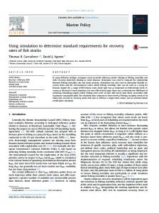
Figure 4.1: Plots of the posterior predictive distribution for game 1116 of the cross validation data. The first five players are members of the New York Knicks the last four are members of the Indiana Pacers. The vertical line represents the difference in score which is -3 for New York and 3 for Indiana which is what we tried to predict. ALLEN HOUSTON

−20

0

20

0.020 0.010

40

−40

−20

0

20

40

60

0

20

40

Difference in Points

LARRY JOHNSON

CHARLES OAKLEY

DALE DAVIS

20

40

60

0.020 0.000

0.010

0.010 0.000 0

−60

−40

−20

0

20

40

−40

−20

0

20



MARK JACKSON

REGGIE MILLER

RIK SMITS

0.020

0.030 20

40

0.000

0.000

0.010

0.010

0.020

0.020 0.010

0


40

0.030


−20

60

0.030

0.030 0.020

0.020 0.010 0.000

−20

0.000

−40

−20


0.030

−40

−40


0.030

−40

0.000

0.000

0.000

0.010

0.010

0.020

0.020

0.030

0.030

PATRICK EWING

0.030

CHRIS CHILDS

−60

−40

−20

0

20


40

−40

−20

0

20

40


33

60

Table 4.2: Percent of correct cross validation predictions Game 19 124 241 434 486 600 772 889 954 1116 total percent

C 1/1 2/2 0/1 2/2 2/2 0/2 2/2 2/2 2/2 13/16 81.2%

PF 2/2 2/2 0/2 0/2 2/2 0/1 1/1 2/2 1/1 2/2 12/17 70.6%

Position PG SF 2/2 2/2 2/2 2/2 0/2 0/1 1/1 2/2 2/2 1/1 0/2 2/2 1/1 1/1 2/2 2/2 2/2 1/1 2/2 0/1 14/18 12/14 77.8% 85.7%

SG 2/2 2/2 0/1 2/2 2/2 2/2 0/2 1/1 1/2 0/2 13/18 72.2%

total 9/9 10/10 0/7 7/9 9/9 4/7 3/7 9/9 7/7 6/9 64/83 77.1%

percent 100% 100% 0% 77.8% 100% 57.1% 42.9% 100% 100% 66.7% 77.1%

dictions, and figure 4.1 presents plots for the posterior predictive distributions of game 1116. Overall, the model correctly picked the winning team 77% of the time. The model performed very poorly for game 241. This game was between Chicago and Miami, two good teams in the 1996-1997 season. Miami beat Chicago by three points, but Michael Jordan dominated the shooting guard position and Scottie Pippen his small forward opponent, so it would seem like Chicago should have won. Most likely a player not represented in the data played a significant role in the outcome of the game. Jordan was so dominant in this game that the model predicted his team to win by 13 points even though they really lost by 3. Other than game 241 the model seemed to fit the data reasonably well.

34

Figure 4.2: Plots of posterior distributions of parameters for assists, steals, turn overs, offensive rebounds, and defensive rebounds for each position Steals 6

10

Assists

SG SF PG

5

PF C

PF C

0

0

1

2

2

3

Density

6 4

Density

4

8

SG SF PG

0.2

0.4

0.6

0.8

0.0

0.2

0.4

0.6


Turn Overs

Offensive Rebounds

0.8

1.0

7


6

0.0

SG SF PG

6

PF C

PF C

4 3

Density

3

0

0

1

1

2

2

Density

4

5

5

SG SF PG

−0.8

−0.7

−0.6

−0.5

−0.4

−0.3

−0.2

−0.1


−0.5

−0.4

−0.3

−0.2

−0.1

0.0

0.1

0.2


10

Defensive Rebounds

2

4

6

PF C

0

Density

8

SG SF PG

0.0

0.2

0.4

0.6

0.8

1.0


35

Figure 4.3: Plots of posterior distributions of parameters for free throws made, free throw percentage,field goals made, and field goal percentage for each position Free Throw Percentage

8

70

Free Throws Made

SG SF PG

60

PF C

PF C

40 0

0

10

2

20

30

Density

4

Density

50

6

SG SF PG

−0.1

0.0

0.1

0.2

0.3

0.4

−0.04

−0.02

0.00

0.02



Field Goals Made

Field Goal Percentage

0.04

8

−0.2

−0.2

−0.1

SG SF PG

40

PF C

PF C

0

10

20

Density

4 2 0

Density

30

6

SG SF PG

−0.3

0.0

0.1


0.2

0.3

0.4

0.00

0.05

0.10

0.15

0.20

0.25

0.30


36

Table 4.3: Posterior means, standard deviations, and 95% highest posterior density credible intervals of parameters of assists, steals, turnovers, free throws made, free throw percentage for each position

4.2

Position Center Power Forward Small Forward Point Guard Shooting Guard

Mean 0.2836 0.3721 0.4013 0.4007 0.4354

Center Power Forward Small Forward Point Guard Shooting Guard

0.5689 0.1908 0.3291 0.2920 0.1957


-0.3648 -0.5687 -0.3912 -0.3764 -0.4281


-0.0041 0.1457 0.1340 0.1468 0.0804


0.0150 -0.0021 -0.0078 -0.0020 –0.0050

Assist(µβ1 ) Std.Dev. 2.5%LHPD 97.5%UHPD 0.0904 0.1151 0.4695 0.0714 0.2269 0.5103 0.0706 0.2600 0.5438 0.0433 0.3135 0.4844 0.0674 0.3032 0.5699 Steals(µβ2 ) 0.1200 0.3252 0.7932 0.1250 -0.0721 0.4268 0.1109 0.0935 0.5316 0.0998 0.0973 0.4955 0.1118 -0.0184 0.4060 Turn Overs(µβ3 ) 0.0805 -0.5186 -0.2072 0.0827 -0.7353 -0.4053 0.0830 -0.5576 -0.2303 0.0782 -0.5345 -0.2304 0.0869 -0.5981 -0.2485 Free Throws Made(µβ4 ) 0.0753 -0.1578 0.1429 0.0690 0.0128 0.2791 0.0711 0.0009 0.2722 0.0672 0.0182 0.2818 0.0669 -0.0541 0.2121 Free Throw Precentage(µβ5 ) 0.0075 0.0007 0.0301 0.0070 -0.0157 0.0115 0.0068 -0.0211 0.0059 0.0067 -0.0153 0.0108 0.0071 -0.0190 0.0087

Positional Summaries

Figures 4.2 and 4.3 provide density plots of the µβh,j ,s. Tables 4.3 and 4.4 contain a summary of the posterior distributions to these parameters. These figures and tables reveal some interesting associations. For all five positions, out-assisting your opponent has a very positive impact

37

Table 4.4: Posterior means, standard deviations, and 95% highest posterior density credible intervals of parameters for field goals made, field goal percentage, offensive rebounds, and defensive rebounds for each of the positions Position Center Power Forward Small Forward Point Guard Shooting Guard

Mean 0.2061 0.0820 0.0508 0.0340 -0.0105


0.0437 0.0700 0.1064 0.1418 0.1703


-0.0911 -0.0152 -0.1492 -0.1391 -0.0913


0.2609 0.3948 0.3530 0.5414 0.4005

Field Goals Made(µβ6 ) Std.Dev. 2.5%LHPD 97.5%UHPD 0.0615 0.0871 0.3259 0.0630 -0.0441 0.2043 0.0723 -0.0933 0.1861 0.0698 -0.0966 0.1795 0.0774 -0.1576 0.1453 Field Goal Percentage(µβ7 ) 0.0118 0.0208 0.0672 0.0136 0.0436 0.0969 0.0153 0.0754 0.1360 0.0153 0.1126 0.1725 0.0185 0.1345 0.2066 Offensive Rebounds(µβ8 ) 0.0634 -0.2147 0.0351 0.0720 -0.1520 0.1279 0.0811 -0.3060 0.0059 0.1234 -0.3990 0.0933 0.1111 -0.3060 0.1228 Defensive Rebounds(µβ9 ) 0.0469 0.1701 0.3535 0.0507 0.2937 0.4944 0.0580 0.2385 0.4646 0.0779 0.3896 0.6974 0.0734 0.2565 0.5481

on a basketball game. A result that is somewhat unexpected is that a shooting guard out-assisting his opponent on average is the most beneficial to the team. A result that we did expect was that a center out-assisting his opponent was the least beneficial. Something that was not expected is how important it is for the center position to record more steals than his opponent. A center that gets one steal more than his opponent gives his team a 0.5689 points advantage on average. In fact, the steals from a center had the largest positive impact among the position

38

box-score category combinations. This association might exist because often times steals from a center occur close to the basket and prevent a potentially easy field goal attempt. In the introduction we hypothesized that a turnover from the point guard would be more detrimental to the team than a turnover from the center position. This did not turn out to be the case. In turns out, a point guard committing one more turnover than the opponent has the least negative effect. A power forward committing one more turnover than the opponent is the most detrimental to a team. It is interesting that a center making more free throws than the opponent is not significant, but shooting a better free throw percentage than the opponent is. The exact opposite holds true for power forwards, small forwards, and point guards. That is, making more free throws than your opponent contributes positively to the outcome of the game, but shooting free throws at a better percentage than your opponent has no impact on the game. This could be attributed to the fact that centers are generally not as proficient at shooting free throws compared to other positions. Because of this, the center could potentially shoot a large number of free throws but make only a few, resulting in a loss of offensive production. Having a better field goal percentage than the opposition is significant for all positions, making more field goals than the opposition is only significant for the center position. Shooting a better field goal percentage than the opposition for players that play a position that requires them to be farther from the basket

39

has the largest effect. Both guards’ field goal percentages have more influence on the outcome of a game than the other positions. This is reasonable because shooting becomes more difficult as the distance between the shooter and the basket increases. Thus having a player that shoots well at these three positions is very beneficial to a team. A very surprising result is that of the offensive rebounds. Most people involved with basketball would agree that an offensive rebound is good, but in this study they are not significant for any position, the effect of out defensive rebounding the positional opponent has a large positive impact on the outcome of the game. The guard positions out-rebounding the opposing guards is more beneficial on average than the remaining three positions. The result that offensive rebounds are insignificant could be a result of the correlation between offensive rebounds and defensive rebounds. If one team is able to get a large number of defensive rebounds then the other team will not be able to get many offensive rebounds. So as one team’s defensive rebounds goes up the other team’s offensive rebounds goes down. In summary, the odds of winning a basketball game increase if all five positions out-rebound, out-assist, and have a better field goal percentage than their positional opponent. So having drills incorporated in their practices that will improve all five positions as defensive rebounders, better shooters, and better distributors of the basketball would increase the chances of winning basketball games. In addition, if centers have drills that will improve their free throw-shooting

40

percentage the odds of winning basketball games improve. Also, power forwards having drills that would improve their passing and dribbling skills to keep their turnovers down would improve a team’s chances of winning. It appears that the small forward position needs to be proficient in all aspects of the game. If their practices incorporate drills that improve shooting percentages, speed, ball handling, strength, and decision-making the probability of winning games would increase. If the guard positions can have a better shooting percentage and outrebound and out-assist their opponents this would be very beneficial to their team and would increase the chances of winning so effective practices for them would include drills that would improve their abilities in these areas.

4.3

Simulation

To ensure that the computer program that implemented the Gibbs sampling algorithm was correct we carried out a simulation study. We generated some NBA box-score data using the proposed model and then we fit the model to the generated data. Since we generated the data we knew what the answers were. By comparing the estimated answers to the generated ones we could monitor the performance of the program. To generate the data we first randomly drew a value from a normal distribution that corresponded to the positional means of the nine regression coefficients for every game that was played. Then, we drew values from an inverse gamma distribution for the variances of the nine regression coefficients, the game effect,

41

team effect, and opponent effect. Then, a game, team, and opponent effect was generated for every game, team, and opponent using a normal distribution with mean zero and variances obtained from the inverse gamma. Next, we generated values for the regression coefficients that corresponded to the player and game being played. This was done by using the values drawn for the positional means and the corresponding variances of the nine β’s as the means and variances of a normal distribution. Next, we took the generated game, team, and opponent effects along with the generated regression coefficient effects and summed these values for each player-game combination. These sums became the means to a normal distribution that will produce the difference in points. Because the players on the same team have the same difference in points, we randomly selected one player from the game and used that player’s sum to obtain a random normal draw. Then the remaining players on the same team as the selected player received the same drawn value for their difference in points and all players on the opposing team received the additive reciprocal for their difference in points. The posterior distribution values that are estimated by the computer program seem to be similar to the generated parameter values. This indicates that the program is performing correctly. Figure 4.4 shows the density plots of a few of the parameters with a vertical line indicating the mean value of the effect from the generated data.

42

Figure 4.4: Plots of the posterior distributions of nine selected parameters using the generated data. The mean of the parameter from generated data is represented by the vertical line µβ13 ast for pg

µβ75 fgm for sg

−10

−5

0

5

10

0.12 0.10 0.08 0.06 0.04 0.02 0.00

0.00

0.00

0.02

0.02

0.04

0.04

0.06

0.06

0.08

0.08

0.10

0.10

0.12

µβ91 drb for c

−10

−5

0

5

10

15

20

−5

10

σβ29 drb

σβ21 ast

σβ27 fgm

10

15

20

0.30 0.20 0.10 0

5

10

15

20

0

5

10

15



σ2

τ5

φ1

0.25

0.30 60

70

0.00

0.00

0.05

0.05

0.10

0.10

0.15

0.15

0.20

0.20

0.25

0.08 0.06 0.04 0.02 0.00

50


20

0.30


40

15

0.00

0.05

0.10

0.15

0.20

0.25

0.30

0.00 0.05 0.10 0.15 0.20 0.25 0.30 0.35


5

30

5


0.00 0

0


−4

−2

0

2


4

6

−4

−2

0

2

4

6


43

Chapter 5

Further Research and Potential Model Improvements

This chapter discusses potential problems that exist in the proposed model and some areas that could produce further research. The chapter can be divided into three sections. The first talks about the importance of players that don’t start. The next section talks about the implicit assumption that interactions are negligible. The last section discusses problems with the current likelihood specification and problems that arise because of how the data are used.

5.1

Bench Players

In the present study, only players that start the game are included in the model. This fails to take into account the impact that the remaining seven players on the team can potentially have on the outcome of a game. Sometimes these players (referred to as bench players) have an important role in the offense. Thus, the association between a successful team and the box-score categories can be confounded with bench play. The bench play can be considered in two ways. One is to include all players and specify the position they play. This will take into

44

account all players but does not give an overall bench effect. The other is to classify all players that don’t start as the bench and treat the bench as a sixth position. This way we can determine how the bench players as a unit need to perform so that their team can be successful. Also, we assumed that each player played the same position for the entire game. This, in reality, is not the case as some players played several positions during the course of a game. To remedy this assumption new data would need to be gathered that identified the position a player was playing each time his team was playing offense.

5.2

Interaction Terms

The model specified is an additive model which implies that all interactions are negligible. That is, all players play the same regardless of where they are playing, and who they are playing with and against. This assumption seems unrealistic. For example, consider the 2005 Phoenix Suns. Prior to the arrival of Steve Nash (a pass first point guard), Amare Stoudamire’s point average was 20.6 points per game with a field goal percentage of 47.5%, while after Nash’s arrival his point average was 26.0 points per game with a field goal percentage of 55.9%. This is a clear case of a player’s performance changing relative to the players on the floor. The model that incorporates interactions would be rather complicated. Graves et al. (2003) modeled interactions between a race track and race car driver. Using an extension of their work would be a good place to start. Fitting a model

45

that contains interaction effects would be very data intense.

5.3

Likelihood and Data Concerns

A consequence of a normal likelihood specification is that the parameter space for a normal density is violated. This is the case because the difference in total points scored is never zero. One way to remedy this would be to disregard overtime periods. That is, take data after 48 minutes regardless if the score is tied or not. Finding data for this model would be very difficult. Another approach would be to specify a new likelihood that would take into account the fact that the response variable can’t be zero. In addition to the likelihood problem the way in which the data were used creates areas of concern. Using each player as an observation required some created dependencies. Instead of treating each player as an observation, each game can be treated as an observation and have a regression term for each position performance category combination. This model would still allow us to estimate positional skills and would eliminate within game dependencies of players from the same team.

5.4

Conclusions

From the results of this study basketball coaches can optimize their odds of winning basketball games by organizing practices that are customized to the needs of each position. In this way, the skills required for each position to reach its potential can be developed. Also, basketball coaches can use the results of the

46

study to build game plans and strategies for specific teams by exploiting positional match-ups. Through developing each position’s skills and building good game plans coaches can increase their chances of winning games.

47

Appendix A

Code Appendix

A.1

FORTRAN code Listing A.1: FORTRAN program to run the MCMC iterations

c c c c

program to p r o d u c e t h e mcmc c r o s s v a l i d a t i o n a n a l y s i s f o r NBA s t u d y u s i n g normal l i k e l i h o o d

i m p l i c i t none i n t e g e r i , j , i i , j j , n , burn , out , l a g , n i t e r , op , g i n t e g e r p l , po , tm , i d i n d e x ( 8 8 4 5 ) , ngames ( 1 3 1 ) , sumobs i n t e g e r DinP ( 8 8 4 5 ) , game ( 8 8 4 5 ) , team ( 8 8 4 5 ) , opp ( 8 8 4 5 ) integer p l a y e r ( 8 8 4 5 ) , pos ( 8 8 4 5 ) r e a l g e n no r , gengam , g e n u n f , z e r o , one , g e n b e t , g e n e x p double p r e c i s i o n f o u l ( 8 8 4 5 ) , a s t ( 8 8 4 5 ) , s t l ( 8 8 4 5 ) , t n o ( 8 8 4 5 ) double p r e c i s i o n p t s ( 8 8 4 5 ) , ftm ( 8 8 4 5 ) , f t p ( 8 8 4 5 ) , fgm ( 8 8 4 5 ) double p r e c i s i o n f g p ( 8 8 4 5 ) , o r b ( 8 8 4 5 ) , drb ( 8 8 4 5 ) double p r e c i s i o n b e t a 0 ( 2 9 ) , mub0 , s i g b 0 double p r e c i s i o n t a u ( 2 9 ) , mut , s i g t double p r e c i s i o n gamma ( 1 1 5 3 ) , mug , s i g g double p r e c i s i o n b e t a 1 ( 1 3 1 ) , mub1 ( 5 ) , s i g b 1 double p r e c i s i o n b e t a 2 ( 1 3 1 ) , mub2 ( 5 ) , s i g b 2 double p r e c i s i o n b e t a 3 ( 1 3 1 ) , mub3 ( 5 ) , s i g b 3 double p r e c i s i o n b e t a 5 ( 1 3 1 ) , mub5 ( 5 ) , s i g b 5 double p r e c i s i o n b e t a 6 ( 1 3 1 ) , mub6 ( 5 ) , s i g b 6 double p r e c i s i o n b e t a 7 ( 1 3 1 ) , mub7 ( 5 ) , s i g b 7 double p r e c i s i o n b e t a 8 ( 1 3 1 ) , mub8 ( 5 ) , s i g b 8 double p r e c i s i o n b e t a 9 ( 1 3 1 ) , mub9 ( 5 ) , s i g b 9 double p r e c i s i o n b e t a 1 0 ( 1 3 1 ) , mub10 ( 5 ) , s i g b 1 0 double p r e c i s i o n mt , s t , at , bt , mg , sg , ag , bg , mb0 , sb0 , ab0 , bb0 double p r e c i s i o n mb1 , mb2 , mb3 , mb5 , mb6 , mb7 , mb8 , mb9 , mb10 double p r e c i s i o n sb1 , sb2 , sb3 , sb5 , sb6 , sb7 , sb8 , sb9 , s b 1 0 double p r e c i s i o n ab1 , ab2 , ab3 , ab5 , ab6 , ab7 , ab8 , ab9 , ab10 double p r e c i s i o n bb1 , bb2 , bb3 , bb5 , bb6 , bb7 , bb8 , bb9 , bb10 double p r e c i s i o n sigma2 , a s i g , b s i g , temp , s o r t ( 8 8 4 5 ) double p r e c i s i o n mub1pos ( 1 3 1 ) , mub2pos ( 1 3 1 ) , mub3pos ( 1 3 1 ) double p r e c i s i o n mub5pos ( 1 3 1 ) , mub6pos ( 1 3 1 ) , mub7pos ( 1 3 1 ) double p r e c i s i o n mub8pos ( 1 3 1 ) , mub9pos ( 1 3 1 ) , mub10pos ( 1 3 1 ) double p r e c i s i o n p o s i t i o n ( 1 3 1 ) e x t e r n a l g e nn o r , gengam , g e n u n f , genexp , g e n b e t , s e t a l l c c c

initialize

assign

starting

values

n i t e r = 20000 call s e t a l l (1090 ,9) do i =1 ,131 b e t a 1 ( i ) =0. d0 b e t a 2 ( i ) =0. d0 b e t a 3 ( i ) =0. d0 b e t a 5 ( i ) =0. d0 b e t a 6 ( i ) =0. d0 b e t a 7 ( i ) =0. d0 b e t a 8 ( i ) =0. d0 b e t a 9 ( i ) =0. d0 b e t a 1 0 ( i ) =0. d0 end do do i = 1 , 2 9

48

b e t a 0 ( i ) =0. d0 t a u ( i ) =0. d0 end do do i =1 ,1153 gamma( i ) =0. d0 end do

do i = 1 , 5 mub1 ( i ) = 0 . d0 mub2 ( i ) = 0 . d0 mub3 ( i ) = 0 . d0 mub5 ( i ) = 0 . d0 mub6 ( i ) = 0 . d0 mub7 ( i ) = 0 . d0 mub8 ( i ) = 0 . d0 mub9 ( i ) = 0 . d0 mub10 ( i ) = 0 . d0 end do s i g m a 2 = 1 . d0 s i g b 0 = 1 . d0 s i g g = 1 . d0 s i g t = 1 . d0 s i g b 1 = 1 . d0 s i g b 2 = 1 . d0 s i g b 3 = 1 . d0 s i g b 5 = 1 . d0 s i g b 6 = 1 . d0 s i g b 7 = 1 . d0 s i g b 8 = 1 . d0 s i g b 9 = 1 . d0 s i g b 1 0 = 1 . d0

c c c

Hyper p r i o r

values

mug = 0 . d0 mut = 0 . d0 mub0 = 0 . d0 at bt

= 1 1 . 0 d0 = 0 . 0 1 1 1 d0

ag bg

= 2 . 4 4 4 4 4 d0 = 0 . 3 4 6 1 5 3 8 d0

ab0 = 1 1 . 0 d0 bb0 = 0 . 0 1 1 1 d0 mb1 = 0 . 0 d0 s b 1 = 2 2 5 . 0 d0 ab1 = 3 . 7 7 7 7 7 8 d0 bb1 = 0 . 0 9 d0 mb2 = 0 . 0 d0 s b 2 = 2 2 5 . 0 d0 ab2 = 3 . 7 7 7 7 7 8 d0 bb2 = 0 . 0 9 d0 mb3 = 0 . 0 d0 s b 3 = 2 2 5 . 0 d0 ab3 = 3 . 7 7 7 7 7 8 d0 bb3 = 0 . 0 9 d0 mb5 = 0 . 0 d0 s b 5 = 2 2 5 . 0 d0 ab5 = 3 . 7 7 7 7 7 8 d0 bb5 = 0 . 0 9 d0 mb6 = 0 . 0 d0 s b 6 = 2 2 5 . 0 d0 ab6 = 3 . 7 7 7 7 7 8 d0 bb6 = 0 . 0 9 d0 mb7 = 0 . 0 d0 s b 7 = 2 2 5 . 0 d0 ab7 = 3 . 7 7 7 7 7 8 d0 bb7 = 0 . 0 9 d0 mb8 = 0 . 0 d0 s b 8 = 2 2 5 . 0 d0 ab8 = 3 . 7 7 7 7 7 8 d0 bb8 = 0 . 0 9 d0 mb9 = 0 . 0 d0 s b 9 = 2 2 5 . 0 d0 ab9 = 3 . 7 7 7 7 7 8 d0 bb9 = 0 . 0 9 d0 mb10 = 0 . 0 d0

49

s b 1 0 = 2 2 5 . 0 d0 ab10 = 3 . 7 7 7 7 7 8 d0 bb10 = 0 . 0 9 d0 a s i g =5.24 d0 b s i g =0.006 d0

burn =50000 out =50000 l a g =2 c c c

read data open ( 1 , f i l e =” n b a c r o s s v a l i d . t x t ” , s t a t u s=” o l d ” ) n=8845 p l =131 po=5 tm=29 op=29 g =1153 do i =1 ,8845 read ( 1 , ∗ ) game ( i ) , DinP ( i ) , p t s ( i ) , a s t ( i ) , o r b ( i ) , drb ( i ) , $ s t l ( i ) , fgm ( i ) , f g p ( i ) , ftm ( i ) , f t p ( i ) , f o u l ( i ) , $ t n o ( i ) , opp ( i ) , team ( i ) , p l a y e r ( i ) , p o s ( i ) end do

c c c

c

c

c c c

c

c c c

open o u t p u t

files

open ( 2 , f i l e =” b e t a 0 . t x t ” , s t a t u s=” unknown ” ) open ( 3 , f i l e =” b e t a 1 . t x t ” , s t a t u s=” unknown ” ) open ( 4 , f i l e =” b e t a 2 . t x t ” , s t a t u s=” unknown ” ) open ( 5 , f i l e =” b e t a 3 . t x t ” , s t a t u s=” unknown ” ) open ( 6 , f i l e =” b e t a 4 . t x t ” , s t a t u s=” unknown” ) open ( 7 , f i l e =” b e t a 5 . t x t ” , s t a t u s=” unknown ” ) open ( 8 , f i l e =” b e t a 6 . t x t ” , s t a t u s=” unknown ” ) open ( 9 , f i l e =” b e t a 7 . t x t ” , s t a t u s=” unknown ” ) open ( 1 0 , f i l e =” b e t a 8 . t x t ” , s t a t u s=” unknown” ) open ( 1 1 , f i l e =” b e t a 9 . t x t ” , s t a t u s=” unknown” ) open ( 1 2 , f i l e =” b e t a 1 0 . t x t ” , s t a t u s=” unknown ” ) open ( 1 3 , f i l e =”mub1 . t x t ” , s t a t u s=” unknown ” ) open ( 1 4 , f i l e =”mub2 . t x t ” , s t a t u s=” unknown ” ) open ( 1 5 , f i l e =”mub3 . t x t ” , s t a t u s=” unknown ” ) open ( 1 6 , f i l e =”mub4 . t x t ” , s t a t u s=” unknown” ) open ( 1 7 , f i l e =”mub5 . t x t ” , s t a t u s=” unknown ” ) open ( 1 8 , f i l e =”mub6 . t x t ” , s t a t u s=” unknown ” ) open ( 1 9 , f i l e =”mub7 . t x t ” , s t a t u s=” unknown ” ) open ( 2 0 , f i l e =”mub8 . t x t ” , s t a t u s=” unknown ” ) open ( 2 1 , f i l e =”mub9 . t x t ” , s t a t u s=” unknown ” ) open ( 2 2 , f i l e =”mub10 . t x t ” , s t a t u s=” unknown” ) open ( 2 3 , f i l e =” t a u . t x t ” , s t a t u s=” unknown” ) open ( 2 4 , f i l e =”gamma . t x t ” , s t a t u s=” unknown” ) open ( 2 5 , f i l e =” s i g m a 2 . t x t ” , s t a t u s=” unknown ” ) open ( 2 6 , f i l e =”mut . t x t ” , s t a t u s=” unknown ” ) open ( 2 7 , f i l e =” s i g t . t x t ” , s t a t u s=” unknown ” ) open ( 2 8 , f i l e =”mugg . t x t ” , s t a t u s=” unknown” ) open ( 2 9 , f i l e =” s i g g . t x t ” , s t a t u s=” unknown ” ) open ( 3 0 , f i l e =”mub0 . t x t ” , s t a t u s=” unknown” ) open ( 3 1 , f i l e =” s i g b 0 . t x t ” , s t a t u s=” unknown” ) open ( 3 2 , f i l e =” s i g b 1 . t x t ” , s t a t u s=” unknown” ) open ( 3 3 , f i l e =” s i g b 2 . t x t ” , s t a t u s=” unknown” ) open ( 3 4 , f i l e =” s i g b 3 . t x t ” , s t a t u s=” unknown” ) open ( 3 5 , f i l e =” s i g b 4 . t x t ” , s t a t u s=” unknown ” ) open ( 3 6 , f i l e =” s i g b 5 . t x t ” , s t a t u s=” unknown” ) open ( 3 7 , f i l e =” s i g b 6 . t x t ” , s t a t u s=” unknown” ) open ( 3 8 , f i l e =” s i g b 7 . t x t ” , s t a t u s=” unknown” ) open ( 3 9 , f i l e =” s i g b 8 . t x t ” , s t a t u s=” unknown” ) open ( 4 0 , f i l e =” s i g b 9 . t x t ” , s t a t u s=” unknown” ) open ( 4 1 , f i l e =” s i g b 1 0 . t x t ” , s t a t u s=” unknown ” )

s t a r t mcmc l o o p

do j j = 1 , ( burn+out ) c c c

compute new v a l u e s

call

for

parameters

getsiggamma ( g , ag , bg , gamma , mug , s i g g )

50

call call

g e t s i g t a u ( op , at , bt , tau , mut , s i g t ) g e t s i g b e t a 0 ( tm , ab0 , bb0 , b e t a 0 , mub0 , s i g b 0 )

call call call call call call call call call

g e t s i g b e t a 1 ( n , ab1 , bb1 , b e t a 1 , p l , mub1pos , s i g b 1 ) g e t s i g b e t a 2 ( n , ab2 , bb2 , b e t a 2 , p l , mub2pos , s i g b 2 ) g e t s i g b e t a 3 ( n , ab3 , bb3 , b e t a 3 , p l , mub3pos , s i g b 3 ) g e t s i g b e t a 5 ( n , ab5 , bb5 , b e t a 5 , p l , mub5pos , s i g b 5 ) g e t s i g b e t a 6 ( n , ab6 , bb6 , b e t a 6 , p l , mub6pos , s i g b 6 ) g e t s i g b e t a 7 ( n , ab7 , bb7 , b e t a 7 , p l , mub7pos , s i g b 7 ) g e t s i g b e t a 8 ( n , ab8 , bb8 , b e t a 8 , p l , mub8pos , s i g b 8 ) g e t s i g b e t a 9 ( n , ab9 , bb9 , b e t a 9 , p l , mub9pos , s i g b 9 ) g e t s i g b e t a 1 0 ( n , ab10 , bb10 , b e t a 1 0 , p l , mub10pos , s i g b 1 0 )

do i i call call call call call call call call call

= 1 ,5 ge t mube t a1 ( i i , n , sb1 , mb1 , b e t a 1 , s i g b 1 , p o s i t i o n , mub1 ( ge t mube t a2 ( i i , n , sb2 , mb2 , b e t a 2 , s i g b 2 , p o s i t i o n , mub2 ( ge t mube t a3 ( i i , n , sb3 , mb3 , b e t a 3 , s i g b 3 , p o s i t i o n , mub3 ( ge t mube t a5 ( i i , n , sb5 , mb5 , b e t a 5 , s i g b 5 , p o s i t i o n , mub5 ( ge t mube t a6 ( i i , n , sb6 , mb6 , b e t a 6 , s i g b 6 , p o s i t i o n , mub6 ( ge t mube t a7 ( i i , n , sb7 , mb7 , b e t a 7 , s i g b 7 , p o s i t i o n , mub7 ( ge t mube t a8 ( i i , n , sb8 , mb8 , b e t a 8 , s i g b 8 , p o s i t i o n , mub8 ( ge t mube t a9 ( i i , n , sb9 , mb9 , b e t a 9 , s i g b 9 , p o s i t i o n , mub9 ( g e t m u b e t a 1 0 ( i i , n , sb10 , mb10 , b e t a 1 0 , s i g b 1 0 , p o s i t i o n , $ mub10 ( i i ) ) end do

$ $ $

$ $ $

$ $ $

ii ii ii ii ii ii ii ii

)) )) )) )) )) )) )) ))

c a l l g e t s i g m a 2 ( i , n , p l a y e r , team , opp , game , DinP , a s t , s t l , tno , ftm , f t p , fgm , f g p , orb , drb , a s i g , b s i g , gamma , tau , b e t a 0 , b e t a 1 , b e t a 2 , b e t a 3 , b e t a 5 , b e t a 6 , b e t a 7 , beta8 , beta9 , beta10 , sigma2 ) do i i = 1 , 1 1 5 3 c a l l getgamma ( i i , n , p l a y e r , team , opp , game , DinP , a s t , s t l , tno , ftm , f t p , fgm , f g p , orb , drb , sigma2 , s i g g , mug , tau , b e t a 0 , beta1 , beta2 , beta3 , beta5 , beta6 , beta7 , beta8 , beta9 , b e t a 1 0 , gamma( i i ) ) end do do i i = 1 , 2 9 c a l l g e t t a u ( i i , n , p l a y e r , team , opp , game , DinP , a s t , s t l , tno , ftm , f t p , fgm , f g p , orb , drb , sigma2 , s i g t , mut , gamma , b e t a 0 , beta1 , beta2 , beta3 , beta5 , beta6 , beta7 , beta8 , beta9 , beta10 , tau ( i i ) ) end do

do i i = 1 , 2 9 c a l l g e t b e t a 0 ( i i , n , p l a y e r , team , opp , game , DinP , a s t , s t l , tno , $ ftm , f t p , fgm , f g p , orb , drb , sigma2 , s i g b 0 , mub0 , gamma , tau , $ beta1 , beta2 , beta3 , beta5 , beta6 , beta7 , beta8 , beta9 , $ beta10 , beta0 ( i i ) ) end do

do i i = 1 , 1 3 1 c a l l g e t b e t a 1 ( i i , n , p l a y e r , team , opp , game , pos , DinP , a s t , s t l , tno , $ ftm , f t p , fgm , f g p , orb , drb , sigma2 , s i g b 1 , mub1 , gamma , tau , $ beta0 , beta2 , beta3 , beta5 , beta6 , beta7 , beta8 , beta9 , $ b e t a 1 0 , p o s i t i o n ( i i ) , mub1pos ( i i ) , b e t a 1 ( i i ) )

$ $ $

c a l l g e t b e t a 2 ( i i , n , p l a y e r , team , opp , game , pos , DinP , a s t , s t l , tno , ftm , f t p , fgm , f g p , orb , drb , sigma2 , s i g b 2 , mub2 , gamma , tau , beta0 , beta1 , beta3 , beta5 , beta6 , beta7 , beta8 , beta9 , b e t a 1 0 , mub2pos ( i i ) , b e t a 2 ( i i ) )

$ $ $


$ $ $


$ $ $


$ $ $


$ $ $


51

$ $ $


$ $ $

c a l l g e t b e t a 1 0 ( i i , n , p l a y e r , team , opp , game , pos , DinP , a s t , s t l , tno , ftm , f t p , fgm , f g p , orb , drb , sigma2 , s i g b 1 0 , mub10 , gamma , tau , beta0 , beta1 , beta2 , beta3 , beta5 , beta6 , beta7 , beta8 , b e t a 9 , mub10pos ( i i ) , b e t a 1 0 ( i i ) ) end do

c c c

write o u t p u t to if ( jj

c

c

c c c

c

c c c

files

. g t . burn ) then

write ( 2 , ∗ ) ( b e t a 0 ( j ) , j = 1 , 2 9 ) write ( 3 , ∗ ) ( b e t a 1 ( j ) , j = 1 , 1 3 1 ) write ( 4 , ∗ ) ( b e t a 2 ( j ) , j = 1 , 1 3 1 ) write ( 5 , ∗ ) ( b e t a 3 ( j ) , j = 1 , 1 3 1 ) write ( 6 , ∗ ) ( b e t a 4 ( j ) , j = 1 , 1 3 1 ) write ( 7 , ∗ ) ( b e t a 5 ( j ) , j = 1 , 1 3 1 ) write ( 8 , ∗ ) ( b e t a 6 ( j ) , j = 1 , 1 3 1 ) write ( 9 , ∗ ) ( b e t a 7 ( j ) , j = 1 , 1 3 1 ) write ( 1 0 , ∗ ) ( b e t a 8 ( j ) , j = 1 , 1 3 1 ) write ( 1 1 , ∗ ) ( b e t a 9 ( j ) , j = 1 , 1 3 1 ) write ( 1 2 , ∗ ) ( b e t a 1 0 ( j ) , j = 1 , 1 3 1 ) write ( 1 3 , ∗ ) ( mub1 ( j ) , j =1 ,5) write ( 1 4 , ∗ ) ( mub2 ( j ) , j =1 ,5) write ( 1 5 , ∗ ) ( mub3 ( j ) , j =1 ,5) write ( 1 6 , ∗ ) ( mub4 ( j ) , j =1 ,5) write ( 1 7 , ∗ ) ( mub5 ( j ) , j =1 ,5) write ( 1 8 , ∗ ) ( mub6 ( j ) , j =1 ,5) write ( 1 9 , ∗ ) ( mub7 ( j ) , j =1 ,5) write ( 2 0 , ∗ ) ( mub8 ( j ) , j =1 ,5) write ( 2 1 , ∗ ) ( mub9 ( j ) , j =1 ,5) write ( 2 2 , ∗ ) ( mub10 ( j ) , j =1 ,5) write ( 2 3 , ∗ ) ( t a u ( j ) , j = 1 , 2 9) write ( 2 4 , ∗ ) (gamma( j ) , j = 1 , 1 1 5 3 ) write ( 2 5 , ∗ ) ( s i g m a 2 ) write ( 2 6 , ∗ ) ( mut ) write ( 2 7 , ∗ ) ( s i g t ) write ( 2 8 , ∗ ) ( mug ) write ( 2 9 , ∗ ) ( s i g g ) write ( 3 0 , ∗ ) ( mub0 ) write ( 3 1 , ∗ ) ( s i g b 0 ) write ( 3 2 , ∗ ) ( s i g b 1 ) write ( 3 3 , ∗ ) ( s i g b 2 ) write ( 3 4 , ∗ ) ( s i g b 3 ) write ( 3 5 , ∗ ) ( s i g b 4 ) write ( 3 6 , ∗ ) ( s i g b 5 ) write ( 3 7 , ∗ ) ( s i g b 6 ) write ( 3 8 , ∗ ) ( s i g b 7 ) write ( 3 9 , ∗ ) ( s i g b 8 ) write ( 4 0 , ∗ ) ( s i g b 9 ) write ( 4 1 , ∗ ) ( s i g b 1 0 ) end i f end mcmc l o o p

end do stop end

c c c c

subroutines

update sigma2 subroutine g e t s i g m a 2 ( i , n , p l a y e r , team , game , opp , DinP , $ a s t , s t l , tno , ftm , f t p , fgm , f g p , orb , drb , a s i g , b s i g , $ gamma , tau , b e t a 0 , b e t a 1 , b e t a 2 , b e t a 3 , b e t a 5 , b e t a 6 , $ beta7 , beta8 , beta9 , beta10 , sigma2 ) i m p l i c i t none i n t e g e r n , i , p l a y e r ( 8 8 4 5 ) , team ( 8 8 4 5 ) , DinP ( 8 8 4 5 ) i n t e g e r opp ( 8 8 4 5 ) , game ( 8 8 4 5 ) double p r e c i s i o n a s t ( 8 8 4 5 ) , s t l ( 8 8 4 5 ) , t n o ( 8 8 4 5 ) , drb ( 8 8 4 5 ) double p r e c i s i o n ftm ( 8 8 4 5 ) , f t p ( 8 8 4 5 ) , fgm ( 8 8 4 5 ) double p r e c i s i o n f g p ( 8 8 4 5 ) , o r b ( 8 8 4 5 ) double p r e c i s i o n b e t a 0 ( 2 9 ) , t a u ( 2 9 ) ,gamma ( 1 1 5 3 ) double p r e c i s i o n b e t a 1 ( 1 3 1 ) , b e t a 2 ( 1 3 1 ) , b e t a 3 ( 1 3 1 ) double p r e c i s i o n b e t a 5 ( 1 3 1 ) , b e t a 6 ( 1 3 1 ) , b e t a 7 ( 1 3 1 )

52

double p r e c i s i o n b e t a 8 ( 1 3 1 ) , b e t a 9 ( 1 3 1 ) , b e t a 1 0 ( 1 3 1 ) double p r e c i s i o n sigma2 , summ , a l l , a s t a r , b s t a r , a s i g , b s i g real rastar , rbstar r e a l gengam e x t e r n a l gengam summ=0. d0 a l l = 0 . d0 do i =1 ,8845 a l l = a l l + 1 . d0 summ = summ + ( d b l e ( DinP ( i ) ) − $ (gamma( game ( i ) ) + t a u ( opp ( i ) ) + b e t a 0 ( team ( i ) ) + $ beta1 ( player ( i ) ) ∗ ast ( i ) + $ beta2 ( player ( i ) ) ∗ s t l ( i ) + $ beta3 ( p l a y e r ( i ) ) ∗ tno ( i ) + $ b e t a 5 ( p l a y e r ( i ) ) ∗ ftm ( i ) + $ beta6 ( player ( i ) ) ∗ f t p ( i ) + $ b e t a 7 ( p l a y e r ( i ) ) ∗fgm ( i ) + $ beta8 ( player ( i ) ) ∗ fgp ( i ) + $ beta9 ( p l a y e r ( i ) ) ∗ orb ( i ) + $ b e t a 1 0 ( p l a y e r ( i ) ) ∗ drb ( i ) ) ) ∗∗2 end do a s t a r = ( a s i g + ( . 5 d0 ) ∗ a l l ) b s t a r = ( ( 1 . d0 / b s i g ) + ( . 5 d0 ) ∗summ) r a s t a r = real ( astar ) rbstar = real ( bstar ) s i g m a 2 = d b l e ( gengam ( r b s t a r , r a s t a r ) ) s i g m a 2 = 1 . d0 / s i g m a 2 end c

u p d a t e gamma t h e i n t e r c e p t f o r t h e gamenumber b e i n g p l a y e d subroutine getgamma ( i i , n , p l a y e r , team , opp , game , DinP , a s t , s t l , $ tno , ftm , f t p , fgm , f g p , orb , drb , sigma2 , s i g g , mug , tau , b e t a 0 , $ beta1 , beta2 , beta3 , beta5 , beta6 , beta7 , beta8 , beta9 , $ b e t a 1 0 , gamma) i m p l i c i t none i n t e g e r n , i , i i , DinP ( 8 8 4 5 ) i n t e g e r p l a y e r ( 8 8 4 5 ) , team ( 8 8 4 5 ) , opp ( 8 8 4 5 ) , game ( 8 8 4 5 ) double p r e c i s i o n a s t ( 8 8 4 5 ) , s t l ( 8 8 4 5 ) , t n o ( 8 8 4 5 ) double p r e c i s i o n drb ( 8 8 4 5 ) , o r b ( 8 8 4 5 ) double p r e c i s i o n fgm ( 8 8 4 5 ) , f g p ( 8 8 4 5 ) , ftm ( 8 8 4 5 ) , f t p ( 8 8 4 5 ) double p r e c i s i o n t a u ( 2 9 ) , b e t a 0 ( 2 9 ) double p r e c i s i o n b e t a 1 ( 1 3 1 ) , b e t a 2 ( 1 3 1 ) , b e t a 3 ( 1 3 1 ) double p r e c i s i o n b e t a 5 ( 1 3 1 ) , b e t a 6 ( 1 3 1 ) , b e t a 7 ( 1 3 1 ) , b e t a 8 ( 1 3 1 ) double p r e c i s i o n b e t a 9 ( 1 3 1 ) , b e t a 1 0 ( 1 3 1 ) double p r e c i s i o n gamma , sigma2 , s i g g , mug double p r e c i s i o n mugamstar , s i g m a 2 g a m s t a r double p r e c i s i o n summ , sumy , sumgamma r e a l z e r o , one real gennor external gennor zero = 0.0 one = 1 . 0 sumy =0. d0 summ=0. d0 sumgamma=0. d0 do i = 1 , 8 8 4 5 i f ( game ( i ) . eq . i i ) then summ = summ+1. d0 sumy = sumy + d b l e ( DinP ( i ) ) sumgamma = sumgamma + $ ( t a u ( opp ( i ) ) + b e t a 0 ( team ( i ) ) + $ beta1 ( player ( i ) ) ∗ ast ( i ) + $ beta2 ( player ( i ) ) ∗ s t l ( i ) + $ beta3 ( p l a y e r ( i ) ) ∗ tno ( i ) + $ b e t a 5 ( p l a y e r ( i ) ) ∗ ftm ( i ) + $ beta6 ( player ( i ) ) ∗ f t p ( i ) + $ b e t a 7 ( p l a y e r ( i ) ) ∗fgm ( i ) + $ beta8 ( player ( i ) ) ∗ fgp ( i ) + $ beta9 ( p l a y e r ( i ) ) ∗ orb ( i ) + $ b e t a 1 0 ( p l a y e r ( i ) ) ∗ drb ( i ) ) end i f end do mugamstar=( s i g g ∗sumy − s i g g ∗sumgamma + s i g m a 2 ∗mug ) / $ ( s i g g ∗summ + s i g m a 2 ) s i g m a 2 g a m s t a r=d s q r t ( ( s i g m a 2 ∗ s i g g ) / ( s i g g ∗summ + s i g m a 2 ) ) gamma = mugamstar+s i g m a 2 g a m s t a r ∗ d b l e ( g e n n o r ( z e r o , one ) ) end

c $ $ $

update tau the i n t e r c e p t f o r opponent subroutine g e t t a u ( i i , n , p l a y e r , team , opp , game , DinP , a s t , s t l , tno , ftm , f t p , fgm , f g p , orb , drb , sigma2 , s i g t , mut , gamma , beta0 , beta1 , beta2 , beta3 , beta5 , beta6 , beta7 , beta8 , beta9 , beta10 , tau ) i m p l i c i t none i n t e g e r n , i , i i , DinP ( 8 8 4 5 ) i n t e g e r p l a y e r ( 8 8 4 5 ) , team ( 8 8 4 5 ) , opp ( 8 8 4 5 ) , game ( 8 8 4 5 ) double p r e c i s i o n a s t ( 8 8 4 5 ) , s t l ( 8 8 4 5 ) , t n o ( 8 8 4 5 ) double p r e c i s i o n drb ( 8 8 4 5 ) , o r b ( 8 8 4 5 ) double p r e c i s i o n fgm ( 8 8 4 5 ) , f g p ( 8 8 4 5 ) , ftm ( 8 8 4 5 ) , f t p ( 8 8 4 5 )

53

double p r e c i s i o n gamma ( 1 1 5 3 ) , b e t a 0 ( 2 9 ) double p r e c i s i o n b e t a 1 ( 1 3 1 ) , b e t a 2 ( 1 3 1 ) , b e t a 3 ( 1 3 1 ) double p r e c i s i o n b e t a 5 ( 1 3 1 ) , b e t a 6 ( 1 3 1 ) , b e t a 7 ( 1 3 1 ) double p r e c i s i o n b e t a 8 ( 1 3 1 ) , b e t a 9 ( 1 3 1 ) , b e t a 1 0 ( 1 3 1 ) double p r e c i s i o n tau , sigma2 , s i g t , mut double p r e c i s i o n mu ta us ta r , s i g m a 2 t a u s t a r double p r e c i s i o n summ , sumy , sumtau r e a l z e r o , one real gennor external gennor zero = 0.0 one = 1 . 0 sumy =0. d0 sumtau =0. d0 summ=0. d0 do i = 1 , 8 8 4 5 i f ( opp ( i ) . eq . i i ) then summ = summ+1. d0 sumy = sumy + d b l e ( DinP ( i ) ) sumtau = sumtau + $ (gamma( game ( i ) ) + b e t a 0 ( team ( i ) ) + $ beta1 ( player ( i ) ) ∗ ast ( i ) + $ beta2 ( player ( i ) ) ∗ s t l ( i ) + $ beta3 ( p l a y e r ( i ) ) ∗ tno ( i ) + $ b e t a 5 ( p l a y e r ( i ) ) ∗ ftm ( i ) + $ beta6 ( player ( i ) ) ∗ f t p ( i ) + $ b e t a 7 ( p l a y e r ( i ) ) ∗fgm ( i ) + $ beta8 ( player ( i ) ) ∗ fgp ( i ) + $ beta9 ( p l a y e r ( i ) ) ∗ orb ( i ) + $ b e t a 1 0 ( p l a y e r ( i ) ) ∗ drb ( i ) ) end i f end do m u t a u s t a r = ( s i g t ∗sumy − s i g t ∗ sumtau + s i g m a 2 ∗mut ) / $ ( s i g t ∗summ + s i g m a 2 ) s i g m a 2 t a u s t a r = d s q r t ( ( s i g m a 2 ∗ s i g t ) / ( s i g t ∗summ+s i g m a 2 ) ) t a u = m u t a u s t a r + ( s i g m a 2 t a u s t a r ) ∗ d b l e ( g e n n o r ( z e r o , one ) ) end

c

u p d a t e b e t a 0 i n t e r c e p t f o r team subroutine g e t b e t a 0 ( i i , n , p l a y e r , team , opp , game , DinP , a s t , s t l , tno , ftm , f t p , fgm , f g p , orb , drb , sigma2 , s i g b 0 , mub0 , gamma , tau , b e t a 1 , b e t a 2 , b e t a 3 , b e t a 5 , b e t a 6 , b e t a 7 , b e t a 8 , b e t a 9 , beta10 , beta0 ) i m p l i c i t none i n t e g e r n , i , i i , DinP ( 8 8 4 5 ) i n t e g e r p l a y e r ( 8 8 4 5 ) , team ( 8 8 4 5 ) , opp ( 8 8 4 5 ) , game ( 8 8 4 5 ) double p r e c i s i o n a s t ( 8 8 4 5 ) , s t l ( 8 8 4 5 ) , t n o ( 8 8 4 5 ) double p r e c i s i o n drb ( 8 8 4 5 ) , o r b ( 8 8 4 5 ) double p r e c i s i o n fgm ( 8 8 4 5 ) , f g p ( 8 8 4 5 ) , ftm ( 8 8 4 5 ) , f t p ( 8 8 4 5 ) double p r e c i s i o n t a u ( 2 9 ) , gamma ( 1 1 5 3 ) double p r e c i s i o n b e t a 1 ( 1 3 1 ) , b e t a 2 ( 1 3 1 ) , b e t a 3 ( 1 3 1 ) double p r e c i s i o n b e t a 5 ( 1 3 1 ) , b e t a 6 ( 1 3 1 ) , b e t a 7 ( 1 3 1 ) , b e t a 8 ( 1 3 1 ) double p r e c i s i o n b e t a 9 ( 1 3 1 ) , b e t a 1 0 ( 1 3 1 ) double p r e c i s i o n b e t a 0 , sigma2 , s i g b 0 , mub0 double p r e c i s i o n m u b e t a 0 s t a r , s i g m a 2 b e t a 0 s t a r double p r e c i s i o n summ , sumy , sumbeta r e a l z e r o , one real gennor external gennor z e r o =0.0 one =1.0 sumy =0. d0 sumbeta =0. d0 summ=0. d0 do i = 1 , 8 8 4 5 i f ( team ( i ) . eq . i i ) then summ = summ + 1 . d0 sumy = sumy + d b l e ( DinP ( i ) ) sumbeta = sumbeta + $ (gamma( game ( i ) ) + t a u ( opp ( i ) ) + $ beta1 ( player ( i ) ) ∗ ast ( i ) + $ beta2 ( player ( i ) ) ∗ s t l ( i ) + $ beta3 ( p l a y e r ( i ) ) ∗ tno ( i ) + $ b e t a 5 ( p l a y e r ( i ) ) ∗ ftm ( i ) + $ beta6 ( player ( i ) ) ∗ f t p ( i ) + $ b e t a 7 ( p l a y e r ( i ) ) ∗fgm ( i ) + $ beta8 ( player ( i ) ) ∗ fgp ( i ) + $ beta9 ( p l a y e r ( i ) ) ∗ orb ( i ) + $ b e t a 1 0 ( p l a y e r ( i ) ) ∗ drb ( i ) ) end i f end do m u b e t a 0 s t a r =( s i g b 0 ∗sumy − s i g b 0 ∗ sumbeta + s i g m a 2 ∗mub0 ) / $ ( s i g b 0 ∗summ + s i g m a 2 ) s i g m a 2 b e t a 0 s t a r=d s q r t ( ( s i g m a 2 ∗ s i g b 0 ) / ( s i g b 0 ∗summ+s i g m a 2 ) ) b e t a 0 = m u b e t a 0 s t a r+s i g m a 2 b e t a 0 s t a r ∗ d b l e ( g e n n o r ( z e r o , one ) ) end $ $ $

c

update beta1

assists

54

subroutine g e t b e t a 1 ( i i , n , p l a y e r , team , opp , game , pos , DinP , a s t , s t l , tno , ftm , f t p , fgm , f g p , orb , drb , sigma2 , s i g b 1 , mub1 , gamma , tau , b e t a 0 , b e t a 2 , b e t a 3 , b e t a 5 , b e t a 6 , b e t a 7 , b e t a 8 , b e t a 9 , b e t a 1 0 , p o s i t i o n , mub1pos , b e t a 1 ) i m p l i c i t none i n t e g e r n , i , i i , p l a y e r ( 8 8 4 5 ) , team ( 8 8 4 5 ) , opp ( 8 8 4 5 ) , game ( 8 8 4 5 ) i n t e g e r p o s ( 8 8 4 5 ) , DinP ( 8 8 4 5 ) double p r e c i s i o n a s t ( 8 8 4 5 ) , s t l ( 8 8 4 5 ) , t n o ( 8 8 4 5 ) double p r e c i s i o n ftm ( 8 8 4 5 ) , f t p ( 8 8 4 5 ) double p r e c i s i o n o r b ( 8 8 4 5 ) , drb ( 8 8 4 5 ) , fgm ( 8 8 4 5 ) , f g p ( 8 8 4 5 ) double p r e c i s i o n gamma ( 1 1 5 3 ) , t a u ( 2 9 ) , b e t a 0 ( 2 9 ) double p r e c i s i o n b e t a 2 ( 1 3 1 ) , b e t a 3 ( 1 3 1 ) , b e t a 5 ( 1 3 1 ) double p r e c i s i o n b e t a 6 ( 1 3 1 ) , b e t a 7 ( 1 3 1 ) , b e t a 8 ( 1 3 1 ) double p r e c i s i o n b e t a 9 ( 1 3 1 ) , b e t a 1 0 ( 1 3 1 ) double p r e c i s i o n sigma2 , s i g b 1 , mub1 ( 5 ) double p r e c i s i o n m u b e t a 1 s t a r , s i g m a 2 b e t a 1 s t a r double p r e c i s i o n sumya , sumbeta , suma double p r e c i s i o n b e t a 1 , mub1pos , p o s i t i o n r e a l g e n no r , one , z e r o external gennor one = 1 . 0 zero = 0.0 sumya =0. d0 sumbeta =0. d0 suma =0. d0 do i = 1 , 8 8 4 5 i f ( p l a y e r ( i ) . eq . i i ) then suma = suma + a s t ( i ) ∗∗2 sumya = sumya + d b l e ( DinP ( i ) ) ∗ a s t ( i ) sumbeta = sumbeta + a s t ( i ) ∗ ( $ gamma( game ( i ) ) + t a u ( opp ( i ) ) + b e t a 0 ( team ( i ) ) + $ beta2 ( player ( i ) ) ∗ s t l ( i ) + $ beta3 ( p l a y e r ( i ) ) ∗ tno ( i ) + $ b e t a 5 ( p l a y e r ( i ) ) ∗ ftm ( i ) + $ beta6 ( player ( i ) ) ∗ f t p ( i ) + $ b e t a 7 ( p l a y e r ( i ) ) ∗fgm ( i ) + $ beta8 ( player ( i ) ) ∗ fgp ( i ) + $ beta9 ( p l a y e r ( i ) ) ∗ orb ( i ) + $ b e t a 1 0 ( p l a y e r ( i ) ) ∗ drb ( i ) ) mub1pos = mub1 ( p o s ( i ) ) p o s i t i o n=p o s ( i ) end i f end do m u b e t a 1 s t a r =( s i g b 1 ∗sumya−s i g b 1 ∗ sumbeta+s i g m a 2 ∗mub1pos ) / $ ( s i g b 1 ∗suma + s i g m a 2 ) s i g m a 2 b e t a 1 s t a r=d s q r t ( ( s i g m a 2 ∗ s i g b 1 ) / ( s i g b 1 ∗suma+s i g m a 2 ) ) b e t a 1=m u b e t a 1 s t a r +( s i g m a 2 b e t a 1 s t a r ) ∗ d b l e ( g e n n o r ( z e r o , one ) ) mub1pos = mub1pos p o s i t i o n=p o s i t i o n end $ $ $

c

update beta2 s t e a l s subroutine g e t b e t a 2 ( i i , n , p l a y e r , team , opp , game , pos , DinP , a s t , s t l , tno , ftm , f t p , fgm , f g p , orb , drb , sigma2 , s i g b 2 , mub2 , gamma , tau , b e t a 0 , b e t a 1 , b e t a 3 , b e t a 5 , b e t a 6 , b e t a 7 , b e t a 8 , b e t a 9 , b e t a 1 0 , mub2pos , b e t a 2 ) i m p l i c i t none i n t e g e r n , i , i i , p o s ( 8 8 4 5 ) , DinP ( 8 8 4 5 ) i n t e g e r p l a y e r ( 8 8 4 5 ) , team ( 8 8 4 5 ) , opp ( 8 8 4 5 ) , game ( 8 8 4 5 ) double p r e c i s i o n a s t ( 8 8 4 5 ) , s t l ( 8 8 4 5 ) , t n o ( 8 8 4 5 ) double p r e c i s i o n ftm ( 8 8 4 5 ) , f t p ( 8 8 4 5 ) double p r e c i s i o n o r b ( 8 8 4 5 ) , drb ( 8 8 4 5 ) , fgm ( 8 8 4 5 ) , f g p ( 8 8 4 5 ) double p r e c i s i o n gamma ( 1 1 5 3 ) , t a u ( 2 9 ) , b e t a 0 ( 2 9 ) double p r e c i s i o n b e t a 1 ( 1 3 1 ) , b e t a 3 ( 1 3 1 ) , b e t a 5 ( 1 3 1 ) double p r e c i s i o n b e t a 6 ( 1 3 1 ) , b e t a 7 ( 1 3 1 ) , b e t a 8 ( 1 3 1 ) , b e t a 9 ( 1 3 1 ) double p r e c i s i o n b e t a 1 0 ( 1 3 1 ) double p r e c i s i o n sigma2 , s i g b 2 , mub2 ( 5 ) double p r e c i s i o n b e t a 2 , mub2pos double p r e c i s i o n m u b e t a 2 s t a r , s i g m a 2 b e t a 2 s t a r double p r e c i s i o n sumya , sumbeta , suma r e a l g e n no r , one , z e r o external gennor one =1.0 z e r o =0.0 sumya =0. d0 sumbeta =0. d0 suma =0. d0 do i = 1 , 8 8 4 5 i f ( p l a y e r ( i ) . eq . i i ) then suma = suma + ( s t l ( i ) ∗ s t l ( i ) ) sumya = sumya + d b l e ( DinP ( i ) ) ∗ s t l ( i ) sumbeta = sumbeta + s t l ( i ) ∗ ( $ gamma( game ( i ) ) + t a u ( opp ( i ) ) + b e t a 0 ( team ( i ) ) + $ beta1 ( p l a y e r ( i ) ) ∗( a s t ( i ) ) + $ beta3 ( p l a y e r ( i ) ) ∗( tno ( i ) ) + $ b e t a 5 ( p l a y e r ( i ) ) ∗ ( ftm ( i ) ) + $ beta6 ( p l a y e r ( i ) ) ∗( f t p ( i ) ) + $ b e t a 7 ( p l a y e r ( i ) ) ∗ ( fgm ( i ) ) + $ beta8 ( p l a y e r ( i ) ) ∗( fgp ( i ) ) + $ $ $

55

beta9 ( p l a y e r ( i ) ) ∗( orb ( i ) ) + b e t a 1 0 ( p l a y e r ( i ) ) ∗ ( drb ( i ) ) ) mub2pos = mub2 ( p o s ( i ) ) end i f end do m u b e t a 2 s t a r =( s i g b 2 ∗sumya − s i g b 2 ∗ sumbeta + s i g m a 2 ∗mub2pos ) / $ ( s i g b 2 ∗suma + s i g m a 2 ) s i g m a 2 b e t a 2 s t a r=d s q r t ( ( s i g m a 2 ∗ s i g b 2 ) / ( s i g b 2 ∗suma+s i g m a 2 ) ) b e t a 2=m u b e t a 2 s t a r+s i g m a 2 b e t a 2 s t a r ∗ d b l e ( g e n n o r ( z e r o , one ) ) mub2pos=mub2pos end

$ $

c

update beta3 t u r n o v e r s subroutine g e t b e t a 3 ( i i , n , p l a y e r , team , opp , game , pos , DinP , a s t , s t l , tno , ftm , f t p , fgm , f g p , orb , drb , sigma2 , s i g b 3 , mub3 , gamma , tau , b e t a 0 , b e t a 1 , b e t a 2 , b e t a 5 , b e t a 6 , b e t a 7 , b e t a 8 , b e t a 9 , b e t a 1 0 , mub3pos , b e t a 3 ) i m p l i c i t none i n t e g e r n , i , i i , p o s ( 8 8 4 5 ) , DinP ( 8 8 4 5 ) i n t e g e r p l a y e r ( 8 8 4 5 ) , team ( 8 8 4 5 ) , opp ( 8 8 4 5 ) , game ( 8 8 4 5 ) double p r e c i s i o n a s t ( 8 8 4 5 ) , s t l ( 8 8 4 5 ) , t n o ( 8 8 4 5 ) double p r e c i s i o n ftm ( 8 8 4 5 ) , f t p ( 8 8 4 5 ) double p r e c i s i o n o r b ( 8 8 4 5 ) , drb ( 8 8 4 5 ) , fgm ( 8 8 4 5 ) , f g p ( 8 8 4 5 ) double p r e c i s i o n gamma ( 1 1 5 3 ) , t a u ( 2 9 ) , b e t a 0 ( 2 9 ) double p r e c i s i o n b e t a 1 ( 1 3 1 ) , b e t a 2 ( 1 3 1 ) , b e t a 5 ( 1 3 1 ) double p r e c i s i o n b e t a 6 ( 1 3 1 ) , b e t a 7 ( 1 3 1 ) , b e t a 8 ( 1 3 1 ) , b e t a 9 ( 1 3 1 ) double p r e c i s i o n b e t a 1 0 ( 1 3 1 ) double p r e c i s i o n b e t a 3 , mub3pos , sigma2 , s i g b 3 , mub3 ( 5 ) double p r e c i s i o n m u b e t a 3 s t a r , s i g m a 2 b e t a 3 s t a r double p r e c i s i o n sumya , sumbeta , suma r e a l g e n no r , one , z e r o external gennor z e r o =0.0 one =1.0 sumya =0. d0 sumbeta =0. d0 suma =0. d0 do i = 1 , 8 8 4 5 i f ( p l a y e r ( i ) . eq . i i ) then suma = suma + ( t n o ( i ) ∗ t n o ( i ) ) sumya = sumya + d b l e ( DinP ( i ) ) ∗ t n o ( i ) sumbeta = sumbeta + t n o ( i ) ∗ ( $ gamma( game ( i ) ) + t a u ( opp ( i ) ) + b e t a 0 ( team ( i ) ) + $ beta1 ( p l a y e r ( i ) ) ∗( a s t ( i ) ) + $ beta2 ( p l a y e r ( i ) ) ∗( s t l ( i ) ) + $ b e t a 5 ( p l a y e r ( i ) ) ∗ ( ftm ( i ) ) + $ beta6 ( p l a y e r ( i ) ) ∗( f t p ( i ) ) + $ b e t a 7 ( p l a y e r ( i ) ) ∗ ( fgm ( i ) ) + $ beta8 ( p l a y e r ( i ) ) ∗( fgp ( i ) ) + $ beta9 ( p l a y e r ( i ) ) ∗( orb ( i ) ) + $ b e t a 1 0 ( p l a y e r ( i ) ) ∗ ( drb ( i ) ) ) mub3pos = mub3 ( p o s ( i ) ) end i f end do m u b e t a 3 s t a r =( s i g b 3 ∗sumya − s i g b 3 ∗ sumbeta + s i g m a 2 ∗mub3pos ) / $ ( s i g b 3 ∗suma + s i g m a 2 ) s i g m a 2 b e t a 3 s t a r=d s q r t ( ( s i g m a 2 ∗ s i g b 3 ) / ( s i g b 3 ∗suma+s i g m a 2 ) ) b e t a 3=m u b e t a 3 s t a r+s i g m a 2 b e t a 3 s t a r ∗ d b l e ( g e n n o r ( z e r o , one ) ) mub3pos = mub3pos end $ $ $

c

u p d a t e b e t a 5 f r e e t h r o w s made subroutine g e t b e t a 5 ( i i , n , p l a y e r , team , opp , game , pos , DinP , a s t , $ s t l , tno , ftm , f t p , fgm , f g p , orb , drb , sigma2 , s i g b 5 , mub5 , $ gamma , tau , b e t a 0 , b e t a 1 , b e t a 2 , b e t a 3 , b e t a 6 , b e t a 7 , b e t a 8 , $ b e t a 9 , b e t a 1 0 , mub5pos , b e t a 5 ) i m p l i c i t none i n t e g e r n , i , i i , p o s ( 8 8 4 5 ) , DinP ( 8 8 4 5 ) i n t e g e r p l a y e r ( 8 8 4 5 ) , team ( 8 8 4 5 ) , opp ( 8 8 4 5 ) , game ( 8 8 4 5 ) double p r e c i s i o n a s t ( 8 8 4 5 ) , s t l ( 8 8 4 5 ) , t n o ( 8 8 4 5 ) double p r e c i s i o n ftm ( 8 8 4 5 ) , f t p ( 8 8 4 5 ) double p r e c i s i o n o r b ( 8 8 4 5 ) , drb ( 8 8 4 5 ) , fgm ( 8 8 4 5 ) , f g p ( 8 8 4 5 ) double p r e c i s i o n gamma ( 1 1 5 3 ) , t a u ( 2 9 ) , b e t a 0 ( 2 9 ) double p r e c i s i o n b e t a 1 ( 1 3 1 ) , b e t a 2 ( 1 3 1 ) , b e t a 3 ( 1 3 1 ) double p r e c i s i o n b e t a 6 ( 1 3 1 ) , b e t a 7 ( 1 3 1 ) , b e t a 8 ( 1 3 1 ) , b e t a 9 ( 1 3 1 ) double p r e c i s i o n b e t a 1 0 ( 1 3 1 ) double p r e c i s i o n b e t a 5 , mub5pos , sigma2 , s i g b 5 , mub5 ( 5 ) double p r e c i s i o n m u b e t a 5 s t a r , s i g m a 2 b e t a 5 s t a r double p r e c i s i o n sumya , sumbeta , suma r e a l g e n no r , one , z e r o external gennor one =1.0 z e r o =0.0 sumya =0. d0 sumbeta =0. d0 suma =0. d0 do i = 1 , 8 8 4 5 i f ( p l a y e r ( i ) . eq . i i ) then suma = suma + ( ftm ( i ) ∗ ftm ( i ) )

56

sumya = sumya + d b l e ( DinP ( i ) ) ∗ ftm ( i ) sumbeta = sumbeta + ftm ( i ) ∗ ( gamma( game ( i ) ) + t a u ( opp ( i ) ) + b e t a 0 ( team ( i ) ) + beta1 ( player ( i ) ) ∗ ast ( i ) + beta2 ( player ( i ) ) ∗ s t l ( i ) + beta3 ( p l a y e r ( i ) ) ∗ tno ( i ) + beta6 ( player ( i ) ) ∗ f t p ( i ) + b e t a 7 ( p l a y e r ( i ) ) ∗fgm ( i ) + beta8 ( player ( i ) ) ∗ fgp ( i ) + beta9 ( p l a y e r ( i ) ) ∗ orb ( i ) + b e t a 1 0 ( p l a y e r ( i ) ) ∗ drb ( i ) ) mub5pos = mub5 ( p o s ( i ) ) end i f end do m u b e t a 5 s t a r =( s i g b 5 ∗sumya − s i g b 5 ∗ sumbeta + s i g m a 2 ∗mub5pos ) / $ ( s i g b 5 ∗suma + s i g m a 2 ) s i g m a 2 b e t a 5 s t a r=d s q r t ( ( s i g m a 2 ∗ s i g b 5 ) / ( s i g b 5 ∗suma+s i g m a 2 ) ) b e t a 5=m u b e t a 5 s t a r+s i g m a 2 b e t a 5 s t a r ∗ d b l e ( g e n n o r ( z e r o , one ) ) mub5pos=mub5pos end

$ $ $ $ $ $ $ $ $

c

u p d a t e b e t a 6 f r e e throw p e r c e n t a g e subroutine g e t b e t a 6 ( i i , n , p l a y e r , team , opp , game , pos , DinP , a s t , $ s t l , tno , ftm , f t p , fgm , f g p , orb , drb , sigma2 , s i g b 6 , mub6 , $ gamma , tau , b e t a 0 , b e t a 1 , b e t a 2 , b e t a 3 , b e t a 5 , b e t a 7 , b e t a 8 , $ b e t a 9 , b e t a 1 0 , mub6pos , b e t a 6 ) i m p l i c i t none i n t e g e r n , i , i i , p o s ( 8 8 4 5 ) , DinP ( 8 8 4 5 ) i n t e g e r p l a y e r ( 8 8 4 5 ) , team ( 8 8 4 5 ) , opp ( 8 8 4 5 ) , game ( 8 8 4 5 ) double p r e c i s i o n a s t ( 8 8 4 5 ) , s t l ( 8 8 4 5 ) , t n o ( 8 8 4 5 ) double p r e c i s i o n ftm ( 8 8 4 5 ) , f t p ( 8 8 4 5 ) double p r e c i s i o n o r b ( 8 8 4 5 ) , drb ( 8 8 4 5 ) , fgm ( 8 8 4 5 ) , f g p ( 8 8 4 5 ) double p r e c i s i o n gamma ( 1 1 5 3 ) , t a u ( 2 9 ) , b e t a 0 ( 2 9 ) double p r e c i s i o n b e t a 1 ( 1 3 1 ) , b e t a 2 ( 1 3 1 ) , b e t a 3 ( 1 3 1 ) double p r e c i s i o n b e t a 5 ( 1 3 1 ) , b e t a 7 ( 1 3 1 ) , b e t a 8 ( 1 3 1 ) , b e t a 9 ( 1 3 1 ) double p r e c i s i o n b e t a 1 0 ( 1 3 1 ) double p r e c i s i o n b e t a 6 , mub6pos , sigma2 , s i g b 6 , mub6 ( 5 ) double p r e c i s i o n m u b e t a 6 s t a r , s i g m a 2 b e t a 6 s t a r double p r e c i s i o n sumya , sumbeta , suma r e a l g e n no r , one , z e r o external gennor one =1.0 z e r o =0.0 sumya =0. d0 sumbeta =0. d0 suma =0. d0 do i = 1 , 8 8 4 5 i f ( p l a y e r ( i ) . eq . i i ) then suma = suma + f t p ( i ) ∗ f t p ( i ) sumya = sumya + d b l e ( DinP ( i ) ) ∗ f t p ( i ) sumbeta = sumbeta + f t p ( i ) ∗ ( $ gamma( game ( i ) ) + t a u ( opp ( i ) ) + b e t a 0 ( team ( i ) ) + $ beta1 ( player ( i ) ) ∗ ast ( i ) + $ beta2 ( player ( i ) ) ∗ s t l ( i ) + $ beta3 ( p l a y e r ( i ) ) ∗ tno ( i ) + $ b e t a 5 ( p l a y e r ( i ) ) ∗ ftm ( i ) + $ b e t a 7 ( p l a y e r ( i ) ) ∗fgm ( i ) + $ beta8 ( player ( i ) ) ∗ fgp ( i ) + $ beta9 ( p l a y e r ( i ) ) ∗ orb ( i ) + $ b e t a 1 0 ( p l a y e r ( i ) ) ∗ drb ( i ) ) mub6pos = mub6 ( p o s ( i ) ) end i f end do m u b e t a 6 s t a r =( s i g b 6 ∗sumya − s i g b 6 ∗ sumbeta + s i g m a 2 ∗mub6pos ) / $ ( s i g b 6 ∗suma + s i g m a 2 ) s i g m a 2 b e t a 6 s t a r=d s q r t ( ( s i g m a 2 ∗ s i g b 6 ) / ( s i g b 6 ∗suma+s i g m a 2 ) ) b e t a 6=m u b e t a 6 s t a r+s i g m a 2 b e t a 6 s t a r ∗ d b l e ( g e n n o r ( z e r o , one ) ) mub6pos=mub6pos end

c $ $ $

u p d a t e b e t a 7 f i e l d g o a l s made subroutine g e t b e t a 7 ( i i , n , p l a y e r , team , opp , game , pos , DinP , a s t , s t l , tno , ftm , f t p , fgm , f g p , orb , drb , sigma2 , s i g b 7 , mub7 , gamma , tau , b e t a 0 , b e t a 1 , b e t a 2 , b e t a 3 , b e t a 5 , b e t a 6 , b e t a 8 , b e t a 9 , b e t a 1 0 , mub7pos , b e t a 7 ) i m p l i c i t none i n t e g e r n , i , i i , p o s ( 8 8 4 5 ) , DinP ( 8 8 4 5 ) i n t e g e r p l a y e r ( 8 8 4 5 ) , team ( 8 8 4 5 ) , opp ( 8 8 4 5 ) , game ( 8 8 4 5 ) double p r e c i s i o n a s t ( 8 8 4 5 ) , s t l ( 8 8 4 5 ) , t n o ( 8 8 4 5 ) double p r e c i s i o n ftm ( 8 8 4 5 ) , f t p ( 8 8 4 5 ) double p r e c i s i o n o r b ( 8 8 4 5 ) , drb ( 8 8 4 5 ) , fgm ( 8 8 4 5 ) , f g p ( 8 8 4 5 ) double p r e c i s i o n gamma ( 1 1 5 3 ) , t a u ( 2 9 ) , b e t a 0 ( 2 9 ) double p r e c i s i o n b e t a 1 ( 1 3 1 ) , b e t a 2 ( 1 3 1 ) , b e t a 3 ( 1 3 1 ) double p r e c i s i o n b e t a 5 ( 1 3 1 ) , b e t a 6 ( 1 3 1 ) , b e t a 8 ( 1 3 1 ) , b e t a 9 ( 1 3 1 ) double p r e c i s i o n b e t a 1 0 ( 1 3 1 ) double p r e c i s i o n b e t a 7 , mub7pos , sigma2 , s i g b 7 , mub7 ( 5 ) double p r e c i s i o n m u b e t a 7 s t a r , s i g m a 2 b e t a 7 s t a r double p r e c i s i o n sumya , sumbeta , suma r e a l g e n no r , one , z e r o

57

external gennor one =1.0 z e r o =0.0 sumya =0. d0 sumbeta =0. d0 suma =0. d0 do i = 1 , 8 8 4 5 i f ( p l a y e r ( i ) . eq . i i ) then suma = suma + fgm ( i ) ∗fgm ( i ) sumya = sumya + d b l e ( DinP ( i ) ) ∗fgm ( i ) sumbeta = sumbeta + fgm ( i ) ∗ ( $ gamma( game ( i ) ) + t a u ( opp ( i ) ) + b e t a 0 ( team ( i ) ) + $ beta1 ( player ( i ) ) ∗ ast ( i ) + $ beta2 ( player ( i ) ) ∗ s t l ( i ) + $ beta3 ( p l a y e r ( i ) ) ∗ tno ( i ) + $ b e t a 5 ( p l a y e r ( i ) ) ∗ ftm ( i ) + $ beta6 ( player ( i ) ) ∗ f t p ( i ) + $ beta8 ( player ( i ) ) ∗ fgp ( i ) + $ beta9 ( p l a y e r ( i ) ) ∗ orb ( i ) + $ b e t a 1 0 ( p l a y e r ( i ) ) ∗ drb ( i ) ) mub7pos = mub7 ( p o s ( i ) ) end i f end do m u b e t a 7 s t a r =( s i g b 7 ∗sumya − s i g b 7 ∗ sumbeta + s i g m a 2 ∗mub7pos ) / $ ( s i g b 7 ∗suma + s i g m a 2 ) s i g m a 2 b e t a 7 s t a r=d s q r t ( ( s i g m a 2 ∗ s i g b 7 ) / ( s i g b 7 ∗suma+s i g m a 2 ) ) b e t a 7=m u b e t a 7 s t a r+s i g m a 2 b e t a 7 s t a r ∗ d b l e ( g e n n o r ( z e r o , one ) ) mub7pos=mub7pos end c

update beta8 f i e l d g o a l p e r c e n t a g e subroutine g e t b e t a 8 ( i i , n , p l a y e r , team , opp , game , pos , DinP , a s t , s t l , tno , ftm , f t p , fgm , f g p , orb , drb , sigma2 , s i g b 8 , mub8 , gamma , tau , b e t a 0 , b e t a 1 , b e t a 2 , b e t a 3 , b e t a 5 , b e t a 6 , b e t a 7 , b e t a 9 , b e t a 1 0 , mub8pos , b e t a 8 ) i m p l i c i t none i n t e g e r n , i , i i , p o s ( 8 8 4 5 ) , DinP ( 8 8 4 5 ) i n t e g e r p l a y e r ( 8 8 4 5 ) , team ( 8 8 4 5 ) , opp ( 8 8 4 5 ) , game ( 8 8 4 5 ) double p r e c i s i o n a s t ( 8 8 4 5 ) , s t l ( 8 8 4 5 ) , t n o ( 8 8 4 5 ) double p r e c i s i o n ftm ( 8 8 4 5 ) , f t p ( 8 8 4 5 ) double p r e c i s i o n o r b ( 8 8 4 5 ) , drb ( 8 8 4 5 ) , fgm ( 8 8 4 5 ) , f g p ( 8 8 4 5 ) double p r e c i s i o n gamma ( 1 1 5 3 ) , t a u ( 2 9 ) , b e t a 0 ( 2 9 ) double p r e c i s i o n b e t a 1 ( 1 3 1 ) , b e t a 2 ( 1 3 1 ) , b e t a 3 ( 1 3 1 ) double p r e c i s i o n b e t a 5 ( 1 3 1 ) , b e t a 6 ( 1 3 1 ) , b e t a 7 ( 1 3 1 ) , b e t a 9 ( 1 3 1 ) double p r e c i s i o n b e t a 1 0 ( 1 3 1 ) double p r e c i s i o n b e t a 8 , mub8pos , sigma2 , s i g b 8 , mub8 ( 5 ) double p r e c i s i o n m u b e t a 8 s t a r , s i g m a 2 b e t a 8 s t a r double p r e c i s i o n sumya , sumbeta , suma r e a l g e n no r , one , z e r o external gennor one =1.0 z e r o =0.0 sumya =0. d0 sumbeta =0. d0 suma =0. d0 do i = 1 , 8 8 4 5 i f ( p l a y e r ( i ) . eq . i i ) then suma = suma + f g p ( i ) ∗ f g p ( i ) sumya = sumya + d b l e ( DinP ( i ) ) ∗ f g p ( i ) sumbeta = sumbeta + f g p ( i ) ∗ ( $ gamma( game ( i ) ) + t a u ( opp ( i ) ) + b e t a 0 ( team ( i ) ) + $ beta1 ( player ( i ) ) ∗ ast ( i ) + $ beta2 ( player ( i ) ) ∗ s t l ( i ) + $ beta3 ( p l a y e r ( i ) ) ∗ tno ( i ) + $ b e t a 5 ( p l a y e r ( i ) ) ∗ ftm ( i ) + $ beta6 ( player ( i ) ) ∗ f t p ( i ) + $ b e t a 7 ( p l a y e r ( i ) ) ∗fgm ( i ) + $ beta9 ( p l a y e r ( i ) ) ∗ orb ( i ) + $ b e t a 1 0 ( p l a y e r ( i ) ) ∗ drb ( i ) ) mub8pos = mub8 ( p o s ( i ) ) end i f end do m u b e t a 8 s t a r =( s i g b 8 ∗sumya − s i g b 8 ∗ sumbeta + s i g m a 2 ∗mub8pos ) / $ ( s i g b 8 ∗suma + s i g m a 2 ) s i g m a 2 b e t a 8 s t a r=d s q r t ( ( s i g m a 2 ∗ s i g b 8 ) / ( s i g b 8 ∗suma+s i g m a 2 ) ) b e t a 8=m u b e t a 8 s t a r+s i g m a 2 b e t a 8 s t a r ∗ d b l e ( g e n n o r ( z e r o , one ) ) mub8pos=mub8pos end $ $ $

c

update beta9 o f f e n s i v e rebounds subroutine g e t b e t a 9 ( i i , n , p l a y e r , team , opp , game , pos , DinP , a s t , $ s t l , tno , ftm , f t p , fgm , f g p , orb , drb , sigma2 , s i g b 9 , mub9 , $ gamma , tau , b e t a 0 , b e t a 1 , b e t a 2 , b e t a 3 , b e t a 5 , b e t a 6 , b e t a 7 , $ b e t a 8 , b e t a 1 0 , mub9pos , b e t a 9 ) i m p l i c i t none i n t e g e r n , i , i i , p o s ( 8 8 4 5 ) , DinP ( 8 8 4 5 ) i n t e g e r p l a y e r ( 8 8 4 5 ) , team ( 8 8 4 5 ) , opp ( 8 8 4 5 ) , game ( 8 8 4 5 ) double p r e c i s i o n a s t ( 8 8 4 5 ) , s t l ( 8 8 4 5 ) , t n o ( 8 8 4 5 ) double p r e c i s i o n ftm ( 8 8 4 5 ) , f t p ( 8 8 4 5 )

58

double p r e c i s i o n o r b ( 8 8 4 5 ) , drb ( 8 8 4 5 ) , fgm ( 8 8 4 5 ) , f g p ( 8 8 4 5 ) double p r e c i s i o n gamma ( 1 1 5 3 ) , t a u ( 2 9 ) , b e t a 0 ( 2 9 ) double p r e c i s i o n b e t a 1 ( 1 3 1 ) , b e t a 2 ( 1 3 1 ) , b e t a 3 ( 1 3 1 ) double p r e c i s i o n b e t a 5 ( 1 3 1 ) , b e t a 6 ( 1 3 1 ) , b e t a 7 ( 1 3 1 ) , b e t a 8 ( 1 3 1 ) double p r e c i s i o n b e t a 1 0 ( 1 3 1 ) double p r e c i s i o n b e t a 9 , mub9pos , sigma2 , s i g b 9 , mub9 ( 5 ) double p r e c i s i o n m u b e t a 9 s t a r , s i g m a 2 b e t a 9 s t a r double p r e c i s i o n sumya , sumbeta , suma r e a l z e r o , one real gennor external gennor z e r o =0.0 one =1.0 sumya =0. d0 sumbeta =0. d0 suma =0. d0 do i = 1 , 8 8 4 5 i f ( p l a y e r ( i ) . eq . i i ) then suma = suma + o r b ( i ) ∗ o r b ( i ) sumya = sumya + d b l e ( DinP ( i ) ) ∗ o r b ( i ) sumbeta = sumbeta + o r b ( i ) ∗ ( $ gamma( game ( i ) ) + t a u ( opp ( i ) ) + b e t a 0 ( team ( i ) ) + $ beta1 ( player ( i ) ) ∗ ast ( i ) + $ beta2 ( player ( i ) ) ∗ s t l ( i ) + $ beta3 ( p l a y e r ( i ) ) ∗ tno ( i ) + $ b e t a 5 ( p l a y e r ( i ) ) ∗ ftm ( i ) + $ beta6 ( player ( i ) ) ∗ f t p ( i ) + $ b e t a 7 ( p l a y e r ( i ) ) ∗fgm ( i ) + $ beta8 ( player ( i ) ) ∗ fgp ( i ) + $ b e t a 1 0 ( p l a y e r ( i ) ) ∗ drb ( i ) ) mub9pos = mub9 ( p o s ( i ) ) end i f end do m u b e t a 9 s t a r =( s i g b 9 ∗sumya−s i g b 9 ∗ sumbeta+s i g m a 2 ∗mub9pos ) / $ ( s i g b 9 ∗suma + s i g m a 2 ) s i g m a 2 b e t a 9 s t a r=d s q r t ( ( s i g m a 2 ∗ s i g b 9 ) / ( s i g b 9 ∗suma + s i g m a 2 ) ) b e t a 9 = m u b e t a 9 s t a r + s i g m a 2 b e t a 9 s t a r ∗ d b l e ( g e n n o r ( z e r o , one ) ) mub9pos=mub9pos end c

update beta10 d e f e n s i v e rebounds subroutine g e t b e t a 1 0 ( i i , n , p l a y e r , team , opp , game , pos , DinP , a s t , $ s t l , tno , ftm , f t p , fgm , f g p , orb , drb , sigma2 , s i g b 1 0 , mub10 , $ gamma , tau , b e t a 0 , b e t a 1 , b e t a 2 , b e t a 3 , b e t a 5 , b e t a 6 , b e t a 7 , $ b e t a 8 , b e t a 9 , mub10pos , b e t a 1 0 ) i m p l i c i t none i n t e g e r n , i , i i , p o s ( 8 8 4 5 ) , DinP ( 8 8 4 5 ) i n t e g e r p l a y e r ( 8 8 4 5 ) , team ( 8 8 4 5 ) , opp ( 8 8 4 5 ) , game ( 8 8 4 5 ) double p r e c i s i o n a s t ( 8 8 4 5 ) , s t l ( 8 8 4 5 ) , t n o ( 8 8 4 5 ) double p r e c i s i o n ftm ( 8 8 4 5 ) , f t p ( 8 8 4 5 ) double p r e c i s i o n o r b ( 8 8 4 5 ) , drb ( 8 8 4 5 ) , fgm ( 8 8 4 5 ) , f g p ( 8 8 4 5 ) double p r e c i s i o n gamma ( 1 1 5 3 ) , t a u ( 2 9 ) , b e t a 0 ( 2 9 ) double p r e c i s i o n b e t a 1 ( 1 3 1 ) , b e t a 2 ( 1 3 1 ) , b e t a 3 ( 1 3 1 ) double p r e c i s i o n b e t a 5 ( 1 3 1 ) , b e t a 6 ( 1 3 1 ) , b e t a 7 ( 1 3 1 ) , b e t a 8 ( 1 3 1 ) double p r e c i s i o n b e t a 9 ( 1 3 1 ) double p r e c i s i o n b e t a 1 0 , sigma2 , s i g b 1 0 , mub10 ( 5 ) double p r e c i s i o n m u b e t a 1 0 s t a r , s i g m a 2 b e t a 1 0 s t a r double p r e c i s i o n sumya , sumbeta , suma , mub10pos r e a l z e r o , one real gennor external gennor z e r o =0.0 one =1.0 sumya =0. d0 sumbeta =0. d0 suma =0. d0 do i = 1 , 8 8 4 5 i f ( p l a y e r ( i ) . eq . i i ) then suma = suma + drb ( i ) ∗ drb ( i ) sumya = sumya + d b l e ( DinP ( i ) ) ∗ drb ( i ) sumbeta = sumbeta + drb ( i ) ∗ ( $ gamma( game ( i ) ) + t a u ( opp ( i ) ) + b e t a 0 ( team ( i ) ) + $ beta1 ( player ( i ) ) ∗ ast ( i ) + $ beta2 ( player ( i ) ) ∗ s t l ( i ) + $ beta3 ( p l a y e r ( i ) ) ∗ tno ( i ) + $ b e t a 5 ( p l a y e r ( i ) ) ∗ ftm ( i ) + $ beta6 ( player ( i ) ) ∗ f t p ( i ) + $ b e t a 7 ( p l a y e r ( i ) ) ∗fgm ( i ) + $ beta8 ( player ( i ) ) ∗ fgp ( i ) + $ beta9 ( p l a y e r ( i ) ) ∗ orb ( i ) ) mub10pos = mub10 ( p o s ( i ) ) end i f end do m u b e t a 1 0 s t a r =( s i g b 1 0 ∗sumya−s i g b 1 0 ∗ sumbeta+s i g m a 2 ∗ mub10pos ) / $ ( s i g b 1 0 ∗suma + s i g m a 2 ) s i g m a 2 b e t a 1 0 s t a r=d s q r t ( ( s i g m a 2 ∗ s i g b 1 0 ) / ( s i g b 1 0 ∗suma+s i g m a 2 ) ) b e t a 1 0=m u b e t a 1 0 s t a r+s i g m a 2 b e t a 1 0 s t a r ∗ d b l e ( g e n n o r ( z e r o , one ) ) mub10pos=mub10pos end

59

c

u p d a t e mu beta1 f o r t h e f i v e p o s i t i o n s subroutine ge t mube t a1 ( i i , n , sb1 , mb1 , b e t a 1 , s i g b 1 , p o s i t i o n , mub1 ) i m p l i c i t none integer i , i i , n , p l j double p r e c i s i o n s i g b 1 , sb1 , mb1 double p r e c i s i o n summ , mub1 , mustarb1 , s i g m a s t a r b 1 double p r e c i s i o n b e t a 1 ( 1 3 1 ) , p o s i t i o n ( 1 3 1 ) r e a l g e nn o r , z e r o , one external gennor zero = 0.0 one = 1 . 0 summ=0. d0 p l j =0.0 do i = 1 , 1 3 1 i f ( p o s i t i o n ( i ) . eq . i i ) then p l j=p l j + 1 summ=summ + b e t a 1 ( i ) end i f end do mustarb1 = ( s b 1 ∗summ + mb1∗ s i g b 1 ) / ( d b l e ( p l j ) ∗ s b 1+s i g b 1 ) s i g m a st a r b 1 = d s q r t ( ( s i g b 1 ∗ sb1 ) /( dble ( p l j ) ∗ sb1 + s i g b 1 ) ) mub1=mustarb1 + s i g m a s t a r b 1 ∗ d b l e ( g e n n o r ( z e r o , one ) ) end

c u p d a t e mu beta2 f o r t h e f i v e p o s i t i o n s subroutine ge t mube t a2 ( i i , n , sb2 , mb2 , b e t a 2 , s i g b 2 , p o s i t i o n , mub2 ) i m p l i c i t none integer i , ii ,n, plj double p r e c i s i o n s i g b 2 , sb2 , mb2 double p r e c i s i o n summ , mub2 , mustarb2 , s i g m a s t a r b 2 double p r e c i s i o n b e t a 2 ( 1 3 1 ) , p o s i t i o n ( 1 3 1 ) r e a l g e n no r , one , z e r o external gennor one =1.0 z e r o =0.0 summ=0. d0 p l j =0.0 do i = 1 , 1 3 1 i f ( p o s i t i o n ( i ) . eq . i i ) then p l j=p l j + 1 summ=summ + b e t a 2 ( i ) end i f end do mustarb2 = ( s b 2 ∗summ + mb2∗ s i g b 2 ) / ( d b l e ( p l j ) ∗ s b 2 + s i g b 2 ) s i g m a st a r b 2 = d s q r t ( ( s i g b 2 ∗ sb2 ) /( dble ( p l j ) ∗ sb2 + s i g b 2 ) ) mub2 = mustarb2 + s i g m a s t a r b 2 ∗ d b l e ( g e n n o r ( z e r o , one ) ) end c u p d a t e mu beta3 subroutine ge t mube t a3 ( i i , n , sb3 , mb3 , b e t a 3 , s i g b 3 , p o s i t i o n , mub3 ) i m p l i c i t none integer i , i i , n , p l j double p r e c i s i o n s i g b 3 , sb3 , mb3 double p r e c i s i o n summ , mub3 , mustarb3 , s i g m a s t a r b 3 double p r e c i s i o n b e t a 3 ( 1 3 1 ) , p o s i t i o n ( 1 3 1 ) r e a l g e n no r , one , z e r o external gennor p l j =0.0 summ=0. d0 do i = 1 , 1 3 1 i f ( p o s i t i o n ( i ) . eq . i i ) then p l j=p l j +1 summ=summ + b e t a 3 ( i ) end i f end do mustarb3 = ( s b 3 ∗summ + mb3∗ s i g b 3 ) / ( d b l e ( p l j ) ∗ s b 3 + s i g b 3 ) s i g m a st a r b 3 = d s q r t ( ( s i g b 3 ∗ sb3 ) /( dble ( p l j ) ∗ sb3 + s i g b 3 ) ) mub3 = mustarb3 + s i g m a s t a r b 3 ∗ d b l e ( g e n n o r ( z e r o , one ) ) end

c u p d a t e mu beta5 subroutine ge t mube t a5 ( i i , n , sb5 , mb5 , b e t a 5 , s i g b 5 , p o s i t i o n , mub5 ) i m p l i c i t none integer i , i i , n , p l j double p r e c i s i o n s i g b 5 , sb5 , mb5 double p r e c i s i o n summ , mub5 , mustarb5 , s i g m a s t a r b 5 double p r e c i s i o n b e t a 5 ( 1 3 1 ) , p o s i t i o n ( 1 3 1 ) r e a l g e n no r , one , z e r o external gennor p l j =0.0 summ=0. d0 do i = 1 , 1 3 1 i f ( p o s i t i o n ( i ) . eq . i i ) then p l j=p l j +1 summ=summ + b e t a 5 ( i ) end i f

60

end do mustarb5 = ( s b 5 ∗summ + mb5∗ s i g b 5 ) / ( d b l e ( p l j ) ∗ s b 5 + s i g b 5 ) s i g m a st a r b 5 = d s q r t ( ( s i g b 5 ∗ sb5 ) /( dble ( p l j ) ∗ sb5 + s i g b 5 ) ) mub5 = mustarb5 + s i g m a s t a r b 5 ∗ d b l e ( g e n n o r ( z e r o , one ) ) end c u p d a t e mu beta6 subroutine ge t mube t a6 ( i i , n , sb6 , mb6 , b e t a 6 , s i g b 6 , p o s i t i o n , mub6 ) i m p l i c i t none integer i , i i , n , p l j double p r e c i s i o n s i g b 6 , sb6 , mb6 double p r e c i s i o n summ , mub6 , mustarb6 , s i g m a s t a r b 6 double p r e c i s i o n b e t a 6 ( 1 3 1 ) , p o s i t i o n ( 1 3 1 ) r e a l g e nn o r , one , z e r o external gennor p l j =0.0 summ=0. d0 do i = 1 , 1 3 1 i f ( p o s i t i o n ( i ) . eq . i i ) then p l j=p l j +1 summ=summ + b e t a 6 ( i ) end i f end do mustarb6 = ( s b 6 ∗summ + mb6∗ s i g b 6 ) / ( d b l e ( p l j ) ∗ s b 6 + s i g b 6 ) s i g m a st a r b 6 = d s q r t ( ( s i g b 6 ∗ sb6 ) /( dble ( p l j ) ∗ sb6 + s i g b 6 ) ) mub6 = mustarb6 + s i g m a s t a r b 6 ∗ d b l e ( g e n n o r ( z e r o , one ) ) end

c u p d a t e mu beta7 subroutine ge t mube t a7 ( i i , n , sb7 , mb7 , b e t a 7 , s i g b 7 , p o s i t i o n , mub7 ) i m p l i c i t none integer i , i i , n , p l j double p r e c i s i o n s i g b 7 , sb7 , mb7 double p r e c i s i o n summ , mub7 , mustarb7 , s i g m a s t a r b 7 double p r e c i s i o n b e t a 7 ( 1 3 1 ) , p o s i t i o n ( 1 3 1 ) r e a l rmsb7 , r s s b 7 r e a l g e n no r , one , z e r o external gennor p l j =0.0 summ=0. d0 do i = 1 , 1 3 1 i f ( p o s i t i o n ( i ) . eq . i i ) then p l j=p l j +1 summ=summ + b e t a 7 ( i ) end i f end do mustarb7 = ( s b 7 ∗summ + mb7∗ s i g b 7 ) / ( d b l e ( p l j ) ∗ s b 7 + s i g b 7 ) s i g m a st a r b 7 = d s q r t ( ( s i g b 7 ∗ sb7 ) /( dble ( p l j ) ∗ sb7 + s i g b 7 ) ) mub7 = mustarb7 + s i g m a s t a r b 7 ∗ d b l e ( g e n n o r ( z e r o , one ) ) end c

u p d a t e mu beta8 subroutine ge t mube t a8 ( i i , n , sb8 , mb8 , b e t a 8 , s i g b 8 , p o s i t i o n , mub8 ) i m p l i c i t none integer i , i i , n , p l j double p r e c i s i o n s i g b 8 , sb8 , mb8 double p r e c i s i o n summ , mub8 , mustarb8 , s i g m a s t a r b 8 double p r e c i s i o n b e t a 8 ( 1 3 1 ) , p o s i t i o n ( 1 3 1 ) r e a l g e nn o r , one , z e r o external gennor p l j =0.0 summ=0. d0 do i = 1 , 1 3 1 i f ( p o s i t i o n ( i ) . eq . i i ) then p l j=p l j +1 summ=summ + b e t a 8 ( i ) end i f end do mustarb8 = ( s b 8 ∗summ + mb8∗ s i g b 8 ) / ( d b l e ( p l j ) ∗ s b 8 + s i g b 8 ) s i g m a st a r b 8 = d s q r t ( ( s i g b 8 ∗ sb8 ) /( dble ( p l j ) ∗ sb8 + s i g b 8 ) ) mub8 = mustarb8 + s i g m a s t a r b 8 ∗ d b l e ( g e n n o r ( z e r o , one ) ) end

c

u p d a t e mu beta9 subroutine ge t mube t a9 ( i i , n , sb9 , mb9 , b e t a 9 , s i g b 9 , p o s i t i o n , mub9 ) i m p l i c i t none integer i , i i , n , p l j double p r e c i s i o n s i g b 9 , sb9 , mb9 double p r e c i s i o n summ , mub9 , mustarb9 , s i g m a s t a r b 9 double p r e c i s i o n b e t a 9 ( 1 3 1 ) , p o s i t i o n ( 1 3 1 ) r e a l g e nn o r , one , z e r o external gennor p l j =0.0 summ=0. d0 do i = 1 , 1 3 1 i f ( p o s i t i o n ( i ) . eq . i i ) then p l j=p l j +1 summ=summ + b e t a 9 ( i )

61

end i f end do mustarb9 =( s b 9 ∗summ+mb9∗ s i g b 9 ) / ( d b l e ( p l j ) ∗ s b 9+s i g b 9 ) s i g m a st a r b 9 = d s q r t ( ( s i g b 9 ∗ sb9 ) /( dble ( p l j ) ∗ sb9 + s i g b 9 ) ) mub9 = mustarb9 + s i g m a s t a r b 9 ∗ d b l e ( g e n n o r ( z e r o , one ) ) end c

u p d a t e mu beta10 subroutine g e t m u b e t a 1 0 ( i i , n , sb10 , mb10 , b e t a 1 0 , s i g b 1 0 , $ p o s i t i o n , mub10 ) i m p l i c i t none integer i , i i , n , p l j double p r e c i s i o n s i g b 1 0 , sb10 , mb10 double p r e c i s i o n summ , mub10 , mustarb10 , s i g m a s t a r b 1 0 double p r e c i s i o n b e t a 1 0 ( 1 3 1 ) , p o s i t i o n ( 1 3 1 ) r e a l g e n no r , one , z e r o external gennor p l j =0.0 summ=0. d0 do i = 1 , 1 3 1 i f ( p o s i t i o n ( i ) . eq . i i ) then p l j=p l j +1 summ=summ + b e t a 1 0 ( i ) end i f end do mustarb10 = ( s b 1 0 ∗summ+mb10∗ s i g b 1 0 ) / ( d b l e ( p l j ) ∗ s b 1 0+s i g b 1 0 ) s i g m a s t a r b 1 0 = d s q r t ( ( s i g b 1 0 ∗ s b 1 0 ) / ( d b l e ( p l j ) ∗ s b 1 0+s i g b 1 0 ) ) mub10 = mustarb10 + s i g m a s t a r b 1 0 ∗ d b l e ( g e n n o r ( z e r o , one ) ) end

c

u p d a t e sig gamma subroutine getsiggamma ( g , ag , bg , gamma , mug , s i g g ) i m p l i c i t none integer g , i double p r e c i s i o n mug , ag , bg double p r e c i s i o n summ , s i g g , a s t a r g , b s t a r g double p r e c i s i o n gamma ( 1 1 5 3 ) real rastarg , rbstarg r e a l gengam e x t e r n a l gengam summ = 0 . d0 do i = 1 , 1 1 5 3 summ = summ + ( gamma( i ) − mug ) ∗∗2 end do a s t a r g = ( ag + ( 0 . 5 d0 ) ∗ d b l e ( g ) ) b s t a r g = ( ( 1 . d0 / bg ) + ( 0 . 5 d0 ) ∗summ) rast arg = real ( astarg ) rbstarg = real ( bstarg ) s i g g = d b l e ( gengam ( r b s t a r g , r a s t a r g ) ) s i g g = 1 . d0 / s i g g end

c

update s i g t a u subroutine g e t s i g t a u ( op , at , bt , tau , mut , s i g t ) i m p l i c i t none i n t e g e r op , i double p r e c i s i o n mut , at , b t double p r e c i s i o n summ , s i g t , a s t a r t , b s t a r t double p r e c i s i o n t a u ( 2 9 ) real rastart , r b s t a r t r e a l gengam e x t e r n a l gengam summ = 0 . d0 do i = 1 , 2 9 summ = summ + ( t a u ( i ) − mut ) ∗∗2 end do a s t a r t = ( a t + ( . 5 d0 ) ∗ d b l e ( op ) ) b s t a r t = ( ( 1 . d0 / b t ) + ( . 5 d0 ) ∗summ) r a s t a r t = real ( a s t a r t ) r b s t a r t = real ( bstart ) s i g t = d b l e ( gengam ( r b s t a r t , r a s t a r t ) ) s i g t = 1 . d0 / s i g t end

c

update s i g b e t a 0 subroutine g e t s i g b e t a 0 ( tm , ab0 , bb0 , b e t a 0 , mub0 , s i g b 0 ) i m p l i c i t none i n t e g e r tm , i double p r e c i s i o n mub0 , ab0 , bb0 double p r e c i s i o n summ , s i g b 0 , a s t a r b 0 , b s t a r b 0 double p r e c i s i o n b e t a 0 ( 2 9 ) real rastarb0 , rbstarb0 r e a l gengam e x t e r n a l gengam summ=0. d0 do i =1 ,29 summ = summ + ( b e t a 0 ( i ) − mub0 ) ∗∗2 end do a s t a r b 0 = ( ab0 + ( . 5 d0 ) ∗ d b l e ( tm ) )

62

b s t a r b 0 = ( ( 1 . d0 / bb0 ) + ( . 5 d0 ) ∗summ) rastarb0 = real ( astarb0 ) rbstarb0 = real ( bstarb0 ) s i g b 0 = d b l e ( gengam ( r b s t a r b 0 , r a s t a r b 0 ) ) s i g b 0 = 1 . d0 / s i g b 0 end

c

update s i g b e t a 1 subroutine g e t s i g b e t a 1 ( n , ab1 , bb1 , b e t a 1 , p l , mub1pos , s i g b 1 ) i m p l i c i t none integer k , n , j , pl , i , counter double p r e c i s i o n mub1 ( 5 ) , ab1 , bb1 double p r e c i s i o n summ , s i g b 1 , a s t a r b 1 , b s t a r b 1 double p r e c i s i o n b e t a 1 ( 1 3 1 ) , mub1pos ( 1 3 1 ) real rastarb1 , rbstarb1 r e a l gengam e x t e r n a l gengam summ=0. d0 do i =1 ,131 summ = summ + ( b e t a 1 ( i ) − mub1pos ( i ) ) ∗∗2 end do a s t a r b 1 = ( ab1 + ( . 5 d0 ) ∗ d b l e ( p l ) ) b s t a r b 1 = ( ( 1 . d0 / bb1 ) + ( . 5 d0 ) ∗summ) rastarb1 = real ( astarb1 ) rbstarb1 = real ( bstarb1 ) s i g b 1 = d b l e ( gengam ( r b s t a r b 1 , r a s t a r b 1 ) ) s i g b 1 = 1 . d0 / s i g b 1 end

c

update s i g b e t a 2 subroutine g e t s i g b e t a 2 ( n , ab2 , bb2 , b e t a 2 , p l , mub2pos , s i g b 2 ) i m p l i c i t none integer n , j , pl , i double p r e c i s i o n ab2 , bb2 double p r e c i s i o n summ , s i g b 2 , a s t a r b 2 , b s t a r b 2 double p r e c i s i o n b e t a 2 ( 1 3 1 ) , mub2pos ( 1 3 1 ) real rastarb2 , rbstarb2 r e a l gengam e x t e r n a l gengam summ=0. d0 do i =1 ,131 summ = summ + ( b e t a 2 ( i ) − mub2pos ( i ) ) ∗∗2 end do a s t a r b 2 = ( ab2 + ( . 5 d0 ) ∗ d b l e ( p l ) ) b s t a r b 2 = ( ( 1 . d0 / bb2 ) + ( . 5 d0 ) ∗summ) rastarb2 = real ( astarb2 ) rbstarb2 = real ( bstarb2 ) s i g b 2 = d b l e ( gengam ( r b s t a r b 2 , r a s t a r b 2 ) ) s i g b 2 = 1 . d0 / s i g b 2 end

c


c

update s i g b e t a 5 subroutine g e t s i g b e t a 5 ( n , ab5 , bb5 , b e t a 5 , p l , mub5pos , s i g b 5 ) i m p l i c i t none integer n , j , pl , i double p r e c i s i o n ab5 , bb5 double p r e c i s i o n summ , s i g b 5 , a s t a r b 5 , b s t a r b 5 double p r e c i s i o n b e t a 5 ( 1 3 1 ) , mub5pos ( 1 3 1 ) real rastarb5 , rbstarb5 r e a l gengam e x t e r n a l gengam summ=0. d0 do i =1 ,131 summ = summ + ( b e t a 5 ( i ) − mub5pos ( i ) ) ∗∗2 end do

63

a s t a r b 5 = ( ab5 + ( . 5 d0 ) ∗ d b l e ( p l ) ) b s t a r b 5 = ( ( 1 . d0 / bb5 ) + ( . 5 d0 ) ∗summ) rastarb5 = real ( astarb5 ) rbstarb5 = real ( bstarb5 ) s i g b 5 = d b l e ( gengam ( r b s t a r b 5 , r a s t a r b 5 ) ) s i g b 5 = 1 . d0 / s i g b 5 end c


c


c


c

update s i g b e t a 9 subroutine g e t s i g b e t a 9 ( n , ab9 , bb9 , b e t a 9 , p l , mub9pos , s i g b 9 ) i m p l i c i t none integer n , j , pl , i double p r e c i s i o n ab9 , bb9 double p r e c i s i o n summ , s i g b 9 , a s t a r b 9 , b s t a r b 9 double p r e c i s i o n b e t a 9 ( 1 3 1 ) , mub9pos ( 1 3 1 ) real rastarb9 , rbstarb9 r e a l gengam e x t e r n a l gengam summ=0. d0 do i =1 ,131 summ = summ + ( b e t a 9 ( i )−mub9pos ( i ) ) ∗∗2 end do a s t a r b 9 = ( ab9 + ( . 5 d0 ) ∗ d b l e ( p l ) )

64

b s t a r b 9 = ( ( 1 . d0 / bb9 ) + ( . 5 d0 ) ∗summ) rastarb9 = real ( astarb9 ) rbstarb9 = real ( bstarb9 ) s i g b 9 = d b l e ( gengam ( r b s t a r b 9 , r a s t a r b 9 ) ) s i g b 9 = 1 . d0 / s i g b 9 end c

update s i g b e t a 1 0 subroutine g e t s i g b e t a 1 0 ( n , ab10 , bb10 , b e t a 1 0 , p l , mub10pos , s i g b 1 0 ) i m p l i c i t none integer n , j , pl , i double p r e c i s i o n ab10 , bb10 double p r e c i s i o n summ , s i g b 1 0 , a s t a r b 1 0 , b s t a r b 1 0 double p r e c i s i o n b e t a 1 0 ( 1 3 1 ) , mub10pos ( 1 3 1 ) real rastarb10 , rbstarb10 r e a l gengam e x t e r n a l gengam summ=0. d0 do i =1 ,131 summ = summ + ( b e t a 1 0 ( i ) − mub10pos ( i ) ) ∗∗2 end do a s t a r b 1 0 = ( ab10 + ( . 5 d0 ) ∗ d b l e ( p l ) ) b s t a r b 1 0 = ( ( 1 . d0 / bb10 ) + ( . 5 d0 ) ∗summ) rastarb10 = real ( astarb10 ) rbstarb10 = real ( bstarb10 ) s i g b 1 0 = d b l e ( gengam ( r b s t a r b 1 0 , r a s t a r b 1 0 ) ) s i g b 1 0 = 1 . d0 / s i g b 1 0 end

A.2

R code

Listing A.2: R code to format data and summarize draws from the joint posterior distribution ## r e a d i n and f o r m a t d a t a ## T h e s e a r e t h e s t a n d a r d i z e d d a t a w i t h t h e gamenumber on them ## POINT GUARD pg