Using a Signature Function To Determine Resonant and Attenuant 2-Cycles In The Smith-Slatkin Population Model John E. Franke Department of Mathematics North Carolina State University Raleigh, NC 27695-8205 e-mail:
[email protected] and Abdul-Aziz Yakubu Department of Mathematics Howard University Washington, DC 20059 e-mail:
[email protected] October 2, 2006 Abstract We study the responses of discretely reproducing populations to periodic ‡uctuations in three parameters: the carrying capacity and two demographic characteristics of the species. We prove that small 2-periodic ‡uctuations of the three parameters generate 2-cyclic oscillations of the population. We develop a signature function for predicting the responses of populations to 2-periodic ‡uctuations. Our signature function is the sign of a weighted sum of the relative strengths of the oscillations of the three parameters. Periodic environments are deleterious for populations when the signature function is negative, while positive signature functions signal favorable environments. We compute the signature function for the Smith-Slatkin model, and use it to determine regions in parameter space that are either favorable or detrimental to the species.
1
1
Introduction
Franke and Yakubu, in a recent paper, used classical parametric single species discrete-time population models to study the responses of populations to periodic ‡uctuations in two parameters, the carrying capacity and the demographic characteristic of the population (growth rate) [19]. In constant environments, many classical discrete-time single species population models have three parameters, the carrying capacity and two demographic characteristics of the species [1-25, 27-43]. Examples of such 3-parameter single species models include the Smith-Slatkin, Hassell, Bobwhite quail and Maynard-Smith models [1, 3-5, 1921, 33-36, 43]. In this paper, we focus on the e¤ects of 2-periodic forcing of the carrying capacity and two demographic characteristics on populations governed by discrete-time models. Many of our arguments are similar to those in the two parameter paper [19] but are more complicated because of the third parameter. Periodic environments are known to be deleterious for populations governed by the logistic di¤erential or di¤erence equations [6, 39]. That is, the average of the resulting oscillations in the periodic environment is less than the average of the carrying capacities in corresponding constant environments (attenuance). Cushing and Henson obtained similar results for 2-periodic monotone models [6]. Elaydi and Sacker [9-12], Franke and Yakubu [15-19], Kocic [27], and Kon [29, 30] have since extended these results to include p periodic Beverton-Holt population models with or without age-structure, where p > 2. These results are known to be model-dependent [6]. However, in almost all the theoretical studies, with only a few exceptions (see [9-12, 19]), only two parameters are periodically forced: the carrying capacity of the species and one demographic characteristic of the species. Unimodal maps under period-2 forcing in two parameters routinely have up to three coexisting 2-cycles (see [31, 38] for examples). We use the SmithSlatkin model to illustrate multiple 2-cycles in maps under period-2 forcing in three parameters. Also, we construct a signature function, Rd , for determining whether the average total biomass is suppressed via attenuant stable 2-cycles or enhanced via resonant stable 2-cycles. As in [19], Rd is the sign of a weighted sum of the relative strengths of the oscillations of carrying capacity and the two demographic characteristics of the species. We use the 3-parameter Smith-Slatkin model to illustrate that, in the presence of periodic forcing, an inverse relationship between the carrying capacity and one of the demographic characteristics of the species can lead to a decrease in the population biomass (attenuance). However, large values of the carrying capacity and one of the demographic characteristics of the species can lead to an increase in the population biomass (resonance). Consequently, a change in relative strengths of oscillations of carrying capacity and at least one of the demographic characteristics of a species is capable of shifting population dynamics from attenuant to resonant cycles and vice versa. It is know that this dramatic shift is not possible in population models with a single ‡uctuating parameter [19, 22, 23]. Section 2 introduces our framework for studying the impact of environmental ‡uctuations on discrete-time population models with three ‡uctuating parame2
ters. In Section 3, we prove that small 2-periodic perturbations of the carrying capacity and the demographic characteristics of the unforced system produce 2-cycle populations. The signature function, Rd , for predicting resonant and attenuant 2-cycles that perturb from the equilibrium given by the carrying capacity of the unforced system is introduced in Section 4. Rd for the Smith-Slatkin model, and regions in parameter space for the support of attenuant or resonant 2-cycles that perturb from the equilibrium given by the carrying capacity are given in Section 5. In Sections 3, 4 and 5, we assume that a 2-cycle must, for small forcing, be close to the carrying capacity. However, the carrying capacity does not have to be the only source of 2-cycles. To compute Rd for the other coexisting 2-cycles, in Sections 6 and 7 we assume that two 2-cycles perturb from (the two di¤erent phases of) a 2-cycle in the unforced model. In Section 6, we prove that small 2-periodic perturbations of a 2-cycle of the unforced system produce two 2-cycle populations. Signature functions, Rd , for 2-species Kolmogorov type discrete-time population models with 2-periodic forcing of 2-cycles are introduced in Section 7. Rd for the SmithSlatkin model, and regions in parameter space for the support of attenuant or resonant coexisting 2-cycles in the model are also given in Section 7. The implications of our results are discussed in Section 8.
2
Population Models With Three Parameters
Theoretical ecology literature is …lled with single species discrete-time population models that have three parameters. Table (I) is a list of speci…c classical examples of population models with three parameters. TABLE I Examples of Three-Parameter Population Models Model Parameters giving stable Reference fk;m;n (x) = carrying capacity, k > 0 1 n Smith-Slatkin(1950) (1+(mk)n )x 1 2 0 < n < 2 or 0 < m < n 1+(mx) k n 2 [3-5, 19-21] Hassell(1954) mkn x 1 0 0; w2 + w3 > 0 and maxf ; g < w2w+w 3 w1 (minf ; g > w2 +w3 ). Also, Equation (2) has an attenuant (a resonant) w1 2-cycle if > 0, w2 + w3 < 0 and minf ; g > w2 +w3 (maxf ; g < w1 ). Consequently, if w2 + w3 6= 0 the model has both attenuant and w2 +w3 resonant cycles. 1 Proof. If w2 + w3 > 0; > 0 and maxf ; g < w2w+w , then w2 + w3 < 3 w1 ; w1 +w2 +w3 < 0; (w1 +w2 +w3 ) < 0 and Rd is negative. Thus, Theorem (8) gives that the 2-cycle is attenuant. Similar arguments establish the rest of the proof.
10
5
2-cycle Perturbation From Unforced Carrying Capacity: Smith-Slatkin Model
In this section, we use our theorems to study the impact of the combined e¤ects of a ‡uctuating carry capacity and demographic characteristics on the average total biomass of populations that are governed by the Smith-Slatkin model (see Table I). Speci…cally, we compute Rd and use it to investigate parameter regimes of attenuance and resonance of the 2-cycle that perturbs from the equilibrium given by the carrying capacity. When the carrying capacity and both of the demographic characteristics are 2-periodically forced, then the classic Smith-Slatkin model becomes x(t + 1) = x(t)
1 + (m(1 + ( 1)t )k(1 + ( 1)t ))n(1+( 1 + (m(1 + ( 1)t )x(t))n(1+( 1)t )
1)t )
:
(5)
From Table 1, in constant environment, the carrying capacity, k, is asymptoti1 n
cally stable when n < 2 or m < k1 n 2 2 : In either of these cases, Corollary (5) predicts a stable 2-cycle in Model (5). Let A = (1 n + 4(mk)n 4(mk)n n + 4(mk)3n (mk)4n n + (mk)4n , B = (mk)n n2 6(mk)2n n 4(mk)3n n + 6(mk)2n + 2(mk)2n n2 + (mk)3n n2 and C = (mk)3n +2(mk)n n ln(mk)+(mk)2n n ln(mk)+n ln(mk): To determine the e¤ects of periodicity on the 2-cycle, we obtain that Rd = sign( (w1 + w2 + w3 )); where
w1
=
w2
=
w3
=
4k(A + B) ; (1 + (mk)n )2 ( 2 2(mk)n + (mk)n n)2 4kn ; 2 2(mk)n + (mk)n n 4k(3(mk)n + 3(mk)2n + 1 + C) : (1 + (mk)n )2 ( 2 2(mk)n + (mk)n n)
When n = 1; w1 = w2 = w3 =
4mk2 ; (2+mk)2 4k 2+mk ; 4k(mk+1+ln(mk)) : 2+mk
If mk + 1 + ln(mk) > 0, > 0; < 0 and < 0; then Rd < 0 and the 2-cycle is attenuant. That is, a periodic environment is detrimental to the species when the ‡uctuations in the carrying capacity are out of phase with the ‡uctuations mk 1 in the demographic characteristics of the species. Since w > w2 = 2+mk , if w1 mk = 2+mk and all the three ‡uctuations are in phase, then Rd > 0 and w2 the 2-cycle is resonant (see FIG. 1).
11
FIG. 1: Regions in the km-plane where w1 ; w2 and w3 are positive and negative for the 2-periodic Smith-Slatkin model, where n = 1: When n = 3, w1 = w2 = w3 = p 3
4k(2m3 k3 1) ; m3 k3 2 12k ; 3 3 m k 2 4k(m3 k3 +1+3 ln(mk)) : m3 k3 2
1 If p < mk < 2; then w1 < 0; w2 > 0 and w3 > 0 (see FIG. 2). If, in addition, 3 2 the ‡uctuations in the carrying capacity are out of phase with the ‡uctuations in the demographic characteristics of the species, then Rd < 0 and the 2-cycle is attenuant. That is, in the presence of periodic forcing, an inverse relationship between the carrying capacity and one of the demographic characteristics p of the species can lead to a decrease in the population biomass. If mk > 3 2; then w1 > 0; w2 < 0 and w3 < 0 (see FIG. 2). If, in addition, the ‡uctuations in the carrying capacity are out of phase with the ‡uctuations in the demographic characteristics of the species, then Rd > 0 and the 2-cycle is resonant. That is, in the presence of periodic forcing, large values of the carrying capacity and one of the demographic characteristics of the species can lead to an increase in the population biomass.
12
FIG. 2: Regions in the km-plane where w1 ; w2 and w3 are positive and negative for the 2-periodic Smith-Slatkin model, where n = 3: As in the case when n = 3; any time n > 2 there is are two hyperbolas, mk = c1 and mk = c2 with c1 < c2 , in the …rst quadrant of the m; k plane such that w1 > 0; w2 < 0 and w3 < 0 above the higher curve and w1 > 0; w2 > 0 and w3 < 0 below the lower curve. This shows that if n > 2 in the Smith-Slatkin model, out of phase forcing of the carrying capacity and the demographic characteristics leads to an increase in the average population biomass whenever km is large. However, if the forcing is in phase and the forcing of the demographic characteristics are strong enough then the average population biomass decreases. In the region where km is small, in phase ‡uctuations of k and n together with out of phase ‡uctuations in m lead to an increase in the average total population biomass.
6
2-Cycle Perturbation From Unforced 2-Cycle: Two Coexisting 2-Cycles
The classic Smith-Slatkin model, a unimodal map, is capable of undergoing period-doubling bifurcations route to chaos. In this section, we illustrate that small 2-periodic perturbations of a 2-cycle of Equation (1), denoted by fx; yg; produce two 2-cycle populations, fx0 ; x1 g and fy 0 ; y 1 g with x0 , y 1 near x and 13
x1 , y 0 near y. These two 2-cycles reduce to the 2-cycle fx; yg in the absence of period-2 forcing in the parameters. Recall that in the absence of period-2 forcing our general model, Equation (1), is fk;m;n (x) = f (P (x)) = xg(P (x)): Unlike the previous sections, we now assume throughout that fk;m;n (x) has a 2-cycle, fx; yg: Next, we proceed as in Corollary 5 and use the Implicit Function Theorem to show that, for small forcing, two coexisting 2-cycles perturb from fx; yg. In this result, F (P ( ; x)) = fk(1
);m(1
);n(1
fk(1+
)
);m(1+ );n(1+ ) (x).
Theorem 11 Assume fk;m;n has a hyperbolic 2-cycle, fx; yg. Then for all su¢ ciently small j j j j and j j, Equation (2) has a pair of 2-cycle populations fx0 = x0 ( ; ; ); x1 = x1 ( ; ; )g and fy 0 = y 0 ( ; ; ); y 1 = y 1 ( ; ; )g where lim
x0 ( ; ; ) = x,
lim
y 1 ( ; ; ) = x,
( ; ; )!(0;0;0)
( ; ; )!(0;0;0)
lim
x1 ( ; ; ) = y;
lim
y 0 ( ; ; ) = y;
( ; ; )!(0;0;0)
( ; ; )!(0;0;0)
and x0 ( ; ; ); x1 ( ; ; ); y 0 ( ; ; ); y 1 ( ; ; )are C 3 with respect to ; and : If the 2-cycle, fx; yg, is locally asymptotically stable (unstable), then the two 2-cycles are locally asymptotically stable (unstable). Proof. F (P ( ; x)) = xg(b k; m; b n b; x)g(e k; m; e n e; xg(b k; m; b n b; x)); b e where k = k(1+ ), m b = m(1+ ), n b = n(1+ ), k = k(1 ), m e = m(1 ) and n e = n(1 ). Thus, F (P (0; x)) = x and F (P (0; y)) = y. The 2-cycle, 2 fx; yg, is a hyperbolic …xed point of fk;m;n if j
2 @fk;m;n @fk;m;n @fk;m;n (x) j=j (x) (y) j6= 1: @x @x @x
Hence, @F @x
= P (0;x)
@fk;m;n @x
(y)
@fk;m;n @x
= (x)
@F @x
P (0;y)
6= 1:
As in the proof of Theorem 4 and Corollary 5, we apply the Implicit Function Theorem at P (0; x) and P (0; y) to get x0 y0
= x0 ( ; ; ) = y0 ( ; ; ) 14
as two 3-parameters families of …xed points of F: Hence, x0 ( ; ; ) and y 0 ( ; ; ) each gives us a 2-cycle for the 2-periodic dynamical system ffk(1
);n(1
);n(1
) (x); fk(1+ );n(1+ );n(1+ ) (x)g:
Let x1 ( ; ; ) = fk(1+
);n(1+ );n(1+ ) (x0 (
; ; ))
y 1 ( ; ; ) = fk(1
);n(1
);n(1
) (y 0 (
; ; )):
);n(1
);n(1
) (x1 (
and Then x0 ( ; ; ) = fk(1 y 0 ( ; ; ) = fk(1+
7
);n(1+ );n(1+
; ; )) and ) (y 1 ( ; ; )):
2-cycle Perturbation From Unforced 2-cycle: Signature Function
In this section, we obtain a signature function, Rd , under the assumption that a 2-cycle must, for small forcing, be close to the 2-cycle fx; yg of Equation (1). When the 2-cycle fx; yg is hyperbolic, Theorem (11) guarantees the four three-parameter families,
x0 ( ; ; ); x1 ( ; ; ); y 0 ( ; ; ) and y 1 ( ; ; ); where x1 ( ; ; ) = fk(1+
);n(1+ );n(1+ ) (x0 (
; ; ))
y 1 ( ; ; ) = fk(1+
);n(1+ );n(1+ ) (y 0 (
; ; )):
and Note that x0 ( ; ; ) = fk(1 y 0 ( ; ; ) = fk(1
);n(1
);n(1
);n(1
);n(1
) (x1 (
; ; )) and (y ( ; ; )): ) 1
Let the linear expansion of these four 3-parameter families about ( ; ; ) = (0; 0; 0) be x0 ( x1 ( y0 ( y1 (
; ; ; ;
; ; ; ;
) ) ) )
x + x01 y + x11 y + y01 x + y11 15
+ x02 + x12 + y02 + y12
+ x03 + x13 + y03 + y13 :
Next, we state the formulas for the coe¢ cients.
x01
=
@F @ P (0;x) @F @x P (0;x) @F @
x02
=
x03
=
1
=
1
@F @x P (0;x)
1
@f @m
=
@f @n
P (y)
+
@f @x
@f @x
@f @x
@f @x
P (y)
@f @m
m
P (y)
;
P (x)
;
1
P (x)
n
P (y)
P (x)
1
P (x)
@f @x
@f @x
@f @k
k
P (y)
P (y)
+
P (y)
=
@f @x
P (y)
@f @x
n P (0;x)
+
P (y) @f @x
m P (0;x)
@F @x P (0;x) @F @
@f @k
k
@f @n
P (x)
;
1
P (x)
and
y01
=
@F @ P (0;y) @F @x P (0;y)
k 1
=
@F @
y02
=
@F @
y03
=
1
@F @x P (0;y)
1
@f @m
=
@f @n
=
P (x)
P (x) @f @x
@f @x
+
@f @x
P (y)
+
@f @x
P (y)
P (x)
@f @x
P (x)
@f @m
m
P (x)
P (x)
16
;
n
P (y)
;
1 @f @n
P (y)
:
1
To get the other 6 coe¢ cients, we let F ( ; ; ; k; m; n; x) = F ( Then F ( ; ; ; k; m; n; x1 ( ; ; )) F ( ; ; ; k; m; n; y 1 ( ; ; ))
P (y)
1
P (x)
@f @x
@f @k
k
P (x) @f @x
P (y)
@f @x
n P (0;y)
+
P (x) @f @x
m
P (0;y) @F @x P (0;y)
@f @k
= x1 ( ; ; ) and = y 1 ( ; ; ):
;
;
; k; m; n; x).
Consequently,
x11
=
@F @ P (0;y) @F @x P (0;y) @F @
x12
=
x13
=
1
=
1
@F @x P (0;y)
1
@f @m
=
@f @n
=
+
P (x)
@f @x @f @x
@f @x
P (y)
@f @m
m
P (x)
;
P (y)
;
1
P (x)
n
P (x)
P (x)
1
P (x)
@f @x
@f @x
@f @k
k
P (y)
P (y)
+
P (x) @f @x
@f @x
P (y)
@f @x
n P (0;y)
+
P (x) @f @x
m P (0;y)
@F @x P (0;y) @F @
@f @k
k
@f @n
P (y)
;
1
P (x)
and
y11
=
@F @ P (0;x) @F @x P (0;x) @F @
y12
=
y13
=
1
1
@F @x P (0;x)
1
@f @m
=
+
P (y) @f @x
@f @n
=
+
P (y)
P (y) @f @x
@f @x
@f @x
P (y)
+
@f @x
P (y)
P (x)
@f @x
P (x)
@f @m
m
P (x)
P (y)
P (x)
;
1
P (y)
@f @x
@f @k
k
P (y) @f @x
P (y)
@f @x
n P (0;x)
@f @k
=
m P (0;x)
@F @x P (0;x) @F @
k
n
P (x)
;
1 @f @n
P (x)
:
1
Let Rd (x) Rd (y)
= w1x + w2x + w3x and = w1y + w2y + w3y ;
where wix = x0i + x1i and wiy = y0i + y1i ; for each i 2 f1; 2; 3g. As in our previous signature function, when the two 2cycles perturb from the 2-cycle in the unforced model, the signature function Rd is a weighted sum of the relative strengths of the oscillations of the carrying capacity and the two demographic characteristic of the species. 17
Lemma 12 Assume fk;m;n has a hyperbolic 2-cycle, fx; yg. Then for all su¢ ciently small j j ; j j and j j, Equation (2) has a pair of 2-cycle populations fx0 = x0 ( ; ; ); x1 = x1 ( ; ; )g and fy 0 = y 0 ( ; ; ); y 1 = y 1 ( ; ; )g; where Rd (x) + Rd (y) = 0: Proof. By Theorem 11, the two coexisting 2-cycles exist. Next, we proceed to show that Rd (x) + Rd (y) = 0: Note that, x01 + x11 + y01 + y11 = @f @f k @f k @f k @f k @f @k jP (y) + @x jP (y) @k jP (x) @k jP (x) + @x jP (x) @k jP (y) @f @f @f @f 1 j j j j @x P (y) @x P (x) @x P (y) @x P (x) 1 @f @f @f @f k @k j + @x j k @k j + @f k @f k @k j @x jP (y) @k jP (x) P (x) P (x) P (y) P (y) @f @f @f @f @x jP (y) @x jP (x) 1 @x jP (y) @x jP (x) 1 = 0: Similarly x02 + x12 + y02 + y12 = 0 and x03 + x13 + y03 + y13 = 0: Hence, Rd (x) + Rd (y) = 0. Note that, Rd (x) + Rd (y) = 0 implies wix = wiy for each i 2 f1; 2; 3g. The next result shows that, typically, one of fx0 ( ; ; ); x1 ( ; ; )g or fy 0 ( ; ; ); y 1 ( ; ; )g is attenuant while the other resonant. Lemma 13 If x01 + x11 6= 0 , x02 + x12 6= 0; and x03 + x13 6= 0; then for each …xed line through the origin in ( ; ; ) space not on the plane Rd (x) = (x01 + x11 ) + (x02 + x12 ) + (x03 + x13 ) = 0 there is a neighborhood of (0; 0; 0) such that on one side fx0 ( ; ; ); x1 ( ; ; )g and fy 0 ( ; ; ); y 1 ( ; ; )g are respectively attenuant and resonant and on the other side they are respectively resonant and attenuant. Proof. To investigate the resonance or attenuance of fx0 ( ; ; ); x1 ( ; ; )g we need to look at x0 ( ; ; ) + x1 ( ; ; ) (x + y) = Rd (x)+ higher order terms. Approaching the origin from one side along a …xed line through the origin in ( ; ; ) space guarantees that the sign of Rd (x) does not change and that it eventually dominates the higher order terms. The sign of Rd (x) changes as we move to the other side of the origin. Thus, if Rd (x) > 0 on one side of the origin, fx0 ( ; ; ); x1 ( ; ; )g is resonant on this side and attenuant on the other side. By the last lemma, Rd (x) = Rd (y) and hence fy 0 ( ; ; ); y 1 ( ; ; )g will be attenuant on the side where fx0 ( ; ; ); x1 ( ; ; )g is resonant and will be resonant on the side where fx0 ( ; ; ); x1 ( ; ; )g is attenuant. Example 14 In the Smith-Slatkin Model with periodic forcing, Equation (5), set the following parameter values. =
=
= 0; k = 2; m = 0:7 and n = 3: 18
Then there is an attracting 2-cycle at f1:2180; 2:8153g: Calculating derivatives at these points we obtain w1x w2x w3x
= x01 + x11 = = x02 + x12 = = x03 + x13 =
9:407036455 + 9:407036504 = 4: 9 10 2:068233172 + 3:665506391 = 1: 597 3 0:750678311 + 2:854772692 = 2: 104 1:
8
By the last lemma, a 2-periodic force applied to this system, usually leads to the emergence of two 2-cycles, where one of them is attenuant and the other is resonant. Another interesting question is to compare the average of all four points on the two 2-cycles with the average of x and y: Since Rd (x) + Rd (y) = 0; the answer to this question comes from a second order form in ( ; ; ): Let Rd (x; y) = w11
2
+ w12
+ w13
+ w22
2
+ w23
+ w33
2
;
where w11 = x011 + x111 + y011 + y111 w12 = x012 + x112 + y012 + y112 w13 = x013 + x113 + y013 + y113 w22 = x022 + x122 + y022 + y122 w23 = x023 + x123 + y023 + y123 w33 = x033 + x133 + y033 + y133 : It is possible for Rd (x; y) to be positive everywhere except at the origin. For example, Rd (x; y) > 0 except at the origin whenever w11 ; w22 ; w33 > 0 and w12 = w13 = w23 = 0. In this case, the four points together generate resonance. It is also possible for Rd (x; y) to be negative everywhere except at the origin. For example, Rd (x; y) < 0 except at the origin whenever w11 ; w22 ; w33 < 0 and w12 = w13 = w23 = 0. In this case, the four points together generate attenuance. In ( ; ; ) space;the sign of Rd (x; y) is constant on any ray starting at the origin. Thus, if Rd (x; y) > 0 for some ( ; ; ), the four points are resonant for some small values of ( ; ; ): For other rays starting at the origin, Rd (x; y) can be negative. Thus, the system can support both resonant and attenuant perturbations. Next, we perturb the previous example and obtain two coexisting stable 2cycles where one is attenuant and the other is resonant. In this example, the four points together are resonant. Example 15 In Example 14, …x all parameters at their current values and set =
=
= 0:01:
As predicted by Theorem 11, the system has two coexisting 2-cycles, a resonant 2-cycle f1:115945; 2:958663g and an attenuant 2-cycle f1:391256; 2:60988g. The 19
average of the four points is 2:0189 and the average of the 2-cycle of the unperturbed system is 2:0166. Hence, together the four points are resonant. Without knowing the coordinates of the two coexisting 2-cycles, one can use Rd (x; y) to determine their attenuance or resonance. To illustrate this, we calculate second partials to determine the following values.
Rd (x; y) = w11 resonant.
8
2
+ w12
w11 = 115 w12 = 150 w13 = 200 w22 = 15 w23 = 36 w33 = 13 + w13 + w22
2
+ w23
+ w33
2
> 0:
As predicted above, Rd (x; y) > 0 and the two 2-cycles together are
Conclusion
Many experimental and theoretical studies predict that populations are either enhanced or suppressed by periodic environments [2, 6, 9-12, 14, 15, 18, 19, 22-27, 29-31, 37, 40-43]. However, in most theoretical studies, with only a few exceptions (see [6, 19, 23, 25, 31, 38]), only the carrying capacity or a demographic characteristic of the species (one or two parameters) are periodically forced. It is known that unimodal maps under period-2 forcing in two model parameters routinely have up to three coexisting 2-cycles [19, 31, 38]. Our results, on population models with three model parameters which are 2-periodically forced, support these predictions. We prove that small 2-periodic ‡uctuations of both the carrying capacity and two demographic characteristics of the species generate 2-cyclic population oscillations. Our results predict both attenuance and resonance in 2-periodically forced, three-parameter population models. As in [19], we derive a signature function, Rd ; for determining the response of discretely reproducing populations to periodic ‡uctuations of their carrying capacity and two demographic characteristics. Rd is the sign of a weighted sum of the relative strengths of the oscillations of the three parameters. Periodic environments are deleterious for the population when Rd is negative, and favorable when Rd is positive. A change in the relative strengths of the environmental and demographic ‡uctuations can shift the system from attenuance to resonance and vice versa. We compute Rd for the Smith-Slatkin model, and determine regions in parameter space where its weights are positive and negative. Once the signs of the weights are known, Rd can be used to decide whether in phase or out of phase forcing of the three parameters is deleterious or bene…cial for the population.
20
When n = 1 and mk is large in the Smith-Slatkin model, a periodic environment is detrimental to the species when the ‡uctuations in the carrying capacity are out of phase with the ‡uctuations in the demographic characteristics of the species. However, when n > 2 and mk is large, these same ‡uctuations lead to an increase in the average population biomass. In constant environments, unimodal maps are capable of supporting 2-cycles. We prove that small 2-periodic perturbations of a 2-cycle of the unforced threeparameter system produce two (coexisting) 2-cycle populations. As in [19], we compute Rd for the coexisting 2-cycles. Usually, one of the 2-cycles will be attenuant and the other will be resonant. We use examples to illustrate attenuant and resonant 2-cycles that perturb from a 2-cycle of the unforced classical Smith-Slatkin model. Our analysis and examples illustrate that, the response of populations to periodic environments is a complex function of the period of the environments, the carrying capacities, all the demographic characteristics of the species, and the type and nature of the ‡uctuations. ACKNOWLEDGEMENT: The authors thank the referees for useful suggestions.
9
References 1. R. J. H. Beverton and S. J. Holt, On the dynamics of exploited …sh populations, H. M. Stationery O¤., London, Fish. Invest., 2, 19 (1957). 2. R. F. Constantino, J. M. Cushing, B. Dennis, R. A. Desharnais and S. M. Henson, Resonant population cycles in temporally ‡uctuating habitats, Bull. Math. Biol. 60, 247-273 (1998). 3. P. Cull, Local and global stability for population models, Biol. Cybern. 54, 141-149 (1986). 4. P. Cull, Stability of discrete one-dimensional population models, Bull. Math. Biol. 50, 1, 67-75 (1988). 5. P. Cull, Stability in one-dimensional models, Scientiae Mathematicae Japonicae, 58, 349-357 (2003). 6. J. M. Cushing and S. M. Henson, Global dynamics of some periodically forced, monotone di¤erence equations, J. Di¤ . Equations Appl. 7, 859872 (2001). 7. S. N. Elaydi, Discrete Chaos. Chapman & Hall/CRC, Boca Raton, FL, 2000. 8. S. N. Elaydi, Periodicity and stability of linear Volterra di¤erence equations, J. Math. Anal. Appl., 181, 483-492 (1994). 21
9. S. N. Elaydi and R. J. Sacker, Global Stability of Periodic Orbits of Nonautonomous Di¤erence Equations and Population Biology, J. Di¤ . Eq. 208 (1), 258-273 (2005). 10. S. N. Elaydi and R. J. Sacker, Global Stability of Periodic Orbits of Nonautonomous Di¤erence Equations In Population Biology and CushingHenson Conjectures, Proceedings of ICDEA8, Brno (2003) (In Press). 11. S. N. Elaydi and R. J. Sacker, Nonautonomous Beverton-Holt Equations and the Cushing-Henson Conjectures, J. Di¤ . Equations Appl (In Press). 12. S. N. Elaydi and R. J. Sacker, Periodic Di¤erence Equations, Populations Biology and the Cushing-Henson Conjectures, (Preprint). 13. S. N. Elaydi and A.-A. Yakubu, Global Stability of Cycles: Lotka-Volterra Competition Model With Stocking, J. Di¤ . Equations Appl. 8(6), 537549 (2002). 14. J. E. Franke and J. F. Selgrade, Attractor for Periodic Dynamical Systems, J. Math. Anal. Appl. 286, 64-79(2003). 15. J. E. Franke and A.-A. Yakubu, Attenuant cycles in periodically forced discrete-time age-structured population models, J. Math. Anal. Appl., 316, 69-86 (2006). 16. J. E. Franke and A.-A. Yakubu, Periodic Dynamical Systems in Unidirectional Metapopulation models, J. Di¤ . Equations Appl., 11(7), 687-700 (2005). 17. J. E. Franke and A.-A. Yakubu, Multiple Attractors Via Cusp Bifurcation In Periodically Varying Environments, J. Di¤ . Equations Appl., 11(4-5), 365-377 (2005). 18. J. E. Franke and A.-A. Yakubu, Population models with periodic recruitment functions and survival rates, J. Di¤ . Equations Appl. 11(14), 11691184 (2005). 19. J. E. Franke and A.-A. Yakubu, Signature Function for Predicting Resonant and Attenuant Population 2-Cycles, Bulletin of Mathematical Biology (In press). 20. M. P. Hassell, Density dependence in single species populations, J. Anim. Ecol. 44, 283-296 (1974) 21. M. P. Hassell, J. H. Lawton and R. M. May, Patterns of dynamical behavior in single species populations, J. Anim. Ecol. 45, 471-486 (1976). 22. S. M. Henson, Multiple attractors and resonance in periodically forced population models, Physics D 140, 33-49 (2000).
22
23. S. M. Henson, The e¤ect of periodicity in maps, J. Di¤ . Equations Appl. 5, 31-56 (1999). 24. S. M. Henson, R. F. Costantino, J. M. Cushing, B. Dennis and R. A. Desharnais, Multiple attractors, saddles, and population dynamics in periodic habitats, Bull. Math. Biol. 61, 1121-1149 (1999). 25. S. M. Henson and J. M. Cushing, The e¤ect of periodic habitat ‡uctuations on a nonlinear insect population model, J. Math. Biol. 36, 201-226 (1997). 26. D. Jillson, Insect populations respond to ‡uctuating environments, Nature, 288, 699-700 (1980). 27. V. L. Kocic, A note on nonautonomous Beverton-Holt model, J. Di¤ . Equations Appl. ( In press). 28. V. L. Kocic and G. Ladas, Global behavior of nonlinear di¤erence equations of higher order with applications, Mathematics and its Applications, 256, Kluwer Academic Publishers Group, Dordrecht, 1993. 29. R. Kon, A note on attenuant cycles of population models with periodic carrying capacity, J. Di¤ . Equations Appl. ( In press). 30. R. Kon, Attenuant cycles of population models with periodic carrying capacity, J. Di¤ . Equations Appl. ( In press). 31. M. Kot and W. M. Scha¤er, The e¤ects of seasonality on discrete models of population growth, Theor. Popl. Biol. 26, 340-360 (1984). 32. J. Li, Periodic solutions of population models in a periodically ‡uctuating environment, Math. Biosc. 110, 17-25 (1992). 33. R. M. May and G. F. Oster, Bifurcations and dynamic complexity in simple ecological models, Amer. Naturalist 110, 573-579 (1976). 34. R. M. May, Simple mathematical models with very complicated dynamics, Nature 261, 459-469 (1977). 35. R. M. May, Stability and complexity in model ecosystems, Princeton University Press (1974). 36. R. M. May, Biological populations with nonoverlapping generations: stable points, stable cycles, and chaos, Science 186, 645-647 (1974). 37. R. M. Nisbet and W. S. C. Gurney, Modelling Fluctuating Populations, Wiley & Son, New York, 1982. 38. D. J. Rodriguez, Models of growth with density regulation in more than one life stage, Theor. Popl. Biol. 34, 93-117 (1988). 39. S. Rosenblat, Population models in a periodically ‡uctuating environment, J. Math. Biol., 9, 23-36 (1980). 23
40. J. F. Selgrade and H. D. Roberds, On the structure of attractors for discrete, periodically forced systems with applications to population models, Physica D 158, 69-82 (2001). 41. J. M. Smith, Models in ecology, Cambridge University Press, Cambridge, England (1974). 42. S. Utida, Population ‡uctuation, an experimental and theoretical approach, Cold Spring Harbor Symp. Quant. Biol. 22, 139-151 (1957). 43. A.-A. Yakubu, Periodically forced nonlinear di¤erence equations with delay, Di¤ erence Equations and Discrete Dynamical Systems, Proceedings of the 9th International Conference, University of Southern California (California, USA), and Editors: L. Allen, B. Aulbach, S. Elaydi and R. Sacker (2005)..
24