Using Complete System Simulation for Temporal Debugging of General Purpose Operating Systems and Workloads Presented at MASCOTS 2000
Lars Albertsson and Peter S Magnusson Computer and Network Architectures Laboratory Swedish Institute of Computer Science Box 1263, SE-164 29 Kista, Sweden
[email protected],
[email protected]
Abstract
price/performance improvements of microprocessor-based computers, in both computation and communication, and the resulting digital convergence of appliances previously not computerized. This trend presses the general purpose desktop computer or server system into service as a soft real-time execution environment, for which it was typically not designed. Specifically, the combined environment of the near future must support applications such as video, audio, games, and control systems along with classic “resource hogs” like word processors and browsers. However, widely used general-purpose operating systems (such as the various flavors of Unix, Windows, and MacOS) are not designed for the needs of real-time applications. Many research efforts have addressed such modifications of existing operating systems. This is a complex task and it is compounded by the lack of adequate tools for real-time system analysis. The debugger is at the heart of toolsets for computer systems programming. However, the correctness of real-time operating systems depends on the time elapsed during execution. Debuggers often interfere with program execution in various ways, and generally lack a notion of temporal correctness. Therefore, the use of conventional debuggers is insufficient for validation of real-time operating systems. Simulator-based debuggers for embedded real-time system design have been in use for some time. Embedded systems have been so much slower than engineering workstations that temporally accurate simulation has been practical using straight-forward implementation techniques. For commodity desktop or server system design, the opposite is true: the user is frequently designing a next-generation high-end system that is faster than any available computer, making the design and implementation of the simulator more difficult. Complete system simulation models an entire target computer at the level of the full instruction set architecture, allowing it to run unmodified commercial operating systems
Digital convergence is precipitating the addition of soft real-time applications to mainstream desktop and server operating environments. Most traditional debuggers for mainstream systems lack a notion of temporal correctness, making them unsuitable for real-time system design and analysis. We propose leveraging complete system simulation to build a temporal debugger capable of analyzing mixed realworld workloads. Traditional real-time system debuggers based on simulation utilize slow, but accurate, simulators. Complete system simulators accept an approximate model of time in exchange for higher performance. The higher performance allows these simulators to analyze high-end commercial operating systems and applications. We describe a temporal debugger design based on complete system simulation and report on some early experiences in analyzing a simple workload. The tool offers a nonintrusive, predictable environment for debugging complex workloads with partial real-time constraints. The simulator foundation allows for interactive debugging of time-critical sequences while preserving a model of execution time flow. Keywords: S OFT R EAL T IME S YSTEMS , T EMPORAL D EBUGGING , O PERATING S YSTEMS , L INUX , S IMICS , C OMPLETE S YSTEM S IMULATION
1. Introduction Applications demanding short response times and throughput guarantees, such as media, entertainment, and telecommunication systems, are increasingly common in general purpose computing environments. This combination — quality of service oriented software competing for resources with mainstream applications — is a relatively new phenomenon. It is a natural result of the ongoing
1
Presented at MASCOTS 2000 Complete system simulators model all the hardware in a system, and only the hardware. As the simulation model is functionally identical to a real system, operating system and application software need not be modified. This limits the sources of errors to those introduced by the hardware model, and by models of simulation input feed. Some significant advances in complete system simulators over the past several years have facilitated the implementation of temporal debuggers. These advances include: efficient instruction set level interpreter kernels [2, 5], mixing levels of temporal accuracy for a given workload [22], extensive support for user annotations [8], and simulator kernels supporting heavy instrumentation [12, 14].
and workloads. Advances in implementation technology allow such simulators to provide a reasonably accurate timing model while executing with a slowdown of roughly 50-200 in relation to native execution [8, 15]. Furthermore, complete system simulators can be designed to be fully deterministic. They thereby effectively address the two major problems in real-time analysis: lack of repeatability and time distortion resulting from intrusion. Also, since simulators are implemented fully in software, they can be freely tailored for specific uses. Simulation thus allow the construction of composite tools for more sophisticated analysis, without interfering with the system under study. The characteristics of complete system simulators therefore make them excellent candidates for building a temporal debugger capable of wrapping an entire target system (including a mix of soft real-time and non-real-time applications) into a single “package” for analysis. With this paper, we propose the use of complete system simulation for temporally correct debugging of a complex mixed workload. We describe the basic functions a simulator-based temporal debugger should implement. We also describe some early work in using such a debugger. Section 2 provides some background regarding complete system simulation and the benefits of using it for real-time analysis. In Section 3, the design of our temporal debugging environment is described. Section 4 presents an early implementation of a simulator-based temporal debugger performing a simple analysis of a real-time workload. Section 5 contains a short survey of related work in real-time analysis and simulation. Conclusions and future work are presented in Section 6.
2.2. Simulation model In order for a simulator to be useful for real-time research, the model provided need not only be functionally correct, but also temporally correct. Thus, it is necessary to account for items affecting execution time at the desired temporal resolution. For large applications, this primarily involves delays from devices, such as disk subsystems, and the memory hierarchy, including the memory management unit (MMU), caches, and memory buses. In general, the accuracy of the temporal model can be compromised without breaking the operating system and applications. It is therefore possible to trade accuracy for speed by using approximative models. The appropriate degree of approximation depends on the size of workload and the time scale of its deadlines. Note that temporal accuracy is less important than predictability and robustness (discussed below). A reasonably accurate time model will provide a coarse understanding of the timing behavior of the system. In order to provide some assurance that a detailed model would not find additional problems, systems can be designed so that margins of error are wider than the granularity of the timing model. Apart from providing a hardware model, an instruction set simulator also provides detailed instrumentation of execution. It records statistics of hardware events associated with the instruction triggering each event. Examples of events recorded by a simulator are: instruction execution count, cache memory misses, and translation look-aside buffer (TLB) misses.
2. Computer system simulation Many design and research areas benefit from simulation of computer systems. Thus, the level of detail provided by simulators range from models of microprocessor chip logic to coarse models of an execution environment including operating system and libraries. In this section, we describe the type of simulator used in the paper and the properties making it useful for real-time analysis.
2.1. Complete system instruction set simulation An important class of simulators provides a model of a machine at the instruction set level, as it represents a welldefined border between hardware and software. Variation of modeling an entire computer system at this level is a traditional theme. This type of simulation has been called “complete machine” [8], “complete computer system” [22], “system level” [13], “instruction set” [2], and “faithful” [5] simulation. In early work, it was referred to as “virtual machines” [4] or simply “simulation” [11]. In this paper we shall use the term “complete system instruction set simulation”, or “complete system simulation”.
2.3. Predictability An artificial system has few unpredictable factors. Thus, a simulated system starting execution in a known state will always execute along the same path. This is useful, both for experiments and debugging, as it is possible to reproduce a state reached in execution. A user of a temporal debugger may detect that excessive time has passed at one point in execution, and restart the simulation to examine recently executed routines more carefully. This is similar to the methodology used for debugging logical correctness of conventional programs. However, as time is part of the state 2
Presented at MASCOTS 2000 the user wishes to verify, it is crucial that temporal behavior is preserved between debugging sessions.
Command line interface
Frontend
2.4. Robustness
Debugger Symbols
In physical systems, measurement of the system generally affects its behavior. This is referred to as the probe effect. Because real-time system analysis tends to focus on short periods of time, even small amounts of temporal intrusion affect measurement quality. This limits both the accuracy and amount of measurement in such systems. Furthermore, the time period under study is too short for a human user to draw conclusions about the correctness of the system. It is not possible to stop execution in order to analyze current state and step carefully forward, which is a common method of debugging conventional systems. In a simulated system, the time scale of the system under study is decoupled from the time scale of the system running the simulator. When the user stops execution, simulation is suspended, and simulated time is frozen. Time distortion due to the probe effect is thereby eliminated. This enables the implementation of a temporal debugger, capable of reporting time as perceived by the application.
Backend
Program Machine
Figure 1. Debugger structure.
tuple consists of an operating system running in a simulated machine. The debugger expects a certain set of primitives needed to probe and control the target machine. Such primitives include reading memory, reading registers, single stepping, and setting breakpoints. Adapting a simulator to the primitives required by a specific debugger enables symbolic debugging of the simulator workload. Unlike traditional debugging environments, such a setup does not impact on execution of the debuggee. Traditional debuggers need to stop the debugged program in order to probe its state, thereby affecting time as perceived by the target program. In addition to primitives required by a debugger frontend, the simulator provides services not normally available in a debugger. Debugger front-ends may allow transparent access to the back-end interface, thereby exporting services not known to the debugger.
2.5. Recording A simulator is built by connecting modules, each representing a hardware device. As mentioned above, these models provide a binary interface to the operating system. However, some device modules also need to interface with the world outside the simulated machine. Such modules may be connected to a corresponding interface in the host environment, for example simulated network interface to a real network, serial line to a terminal emulator, screen to an X window and so on. However, input from the outside world is inherently unpredictable. In order to maintain simulation predictability, modules connecting to the real world record and timestamp all events, enabling exact repetition of the session.
3.2. Temporal debugging The service most relevant for real-time analysis is the ability to present current time with cycle count granularity. It enables the user to step through a portion of code, checking for both functional and temporal errors. Methodology for temporal debugging is similar to debugging conventional applications. The user starts execution, browsing through program flow until an invalid state has been reached. Debugging is then restarted, and the user steps more slowly through routines suspected of causing the error. However, in the case of temporal debugging, state correctness includes the simulated time value.
3. Temporal debugger environment In this section, we describe our design of a temporal debugger. We explain how a debugger is connected to a simulator and provide some details on a temporal debugger setup. We also describe some services the user interface should support in order to provide a complete time-aware debugger environment.
3.3. Real-time performance debugging with instrumented simulation The method described above assumes that the user eventually will discover an erroneous piece of code. This piece of code is assumed to take an undesired execution path, or to set the program in an undesired state, affecting later execution. This assumption is reasonable for conventional applications. However, it is not always true for real-time systems, as time spent in a specific routine may be different between executions, even though program state and input is identical. This is due to the fact that application performance is dependent on stochastic hardware elements, such as cache or TLB contents. Thus, the time elapsed for a part
3.1. Debugging using a simulator back-end A complete debugger setup consists of the debugger program and a target machine running the debugged program. Figure 1 shows the different parts of a debugger setup. We refer to the debugger program itself as front-end and to the target machine/program tuple as back-end. Examples of such tuples are: Unix programs running in the virtual machine provided by the operating system, or an embedded operating system on a separate target board. In our case the 3
Presented at MASCOTS 2000 of program execution is also dependent on hardware state. In order to obtain clues about performance hazards caused by cache effects, the instrumentation provided by the simulator may be consulted. The simulator presents statistics of hardware events, associated with instruction address. In case the time elapsed differs in similar execution paths of a program, aspects such as cache miss counts can be compared to find instructions causing intermittent cache behavior.
Workload
Recorded or synthetic models
simulated console
real
Operating System
Disk Ethernet TTY MMU Caches
Script Lang
Simics
Command line interface
Symbols
local network workload and OS symbol files
3.4. Simics target disk dumps
The simulator used for this work is Virtutech Simics [24]. Simics simulates the SPARC V9 instruction set and models single or multiprocessor systems corresponding to the sun4u architecture from Sun Microsystems, for example the Enterprise 3500. Simics consists of a core interpreter that offers basic services such as an instruction set interpreter, a general event model, and a module for simulating and profiling memory activity. A programming interface allows the addition of device models, which may choose to connect to the “real world” or models thereof, as described in section 2.5. Simics supports a simple time model in its default configuration. This model approximates time by defining a cycle as either an executed instruction, a taken trap, or a part of a memory or device stall. In this mode, Simics thus has a rather simple view of the timing of a modern system, and assumes a linear penalty for events such as TLB miss, data cache miss, and instruction cache miss.
Figure 2. Temporal debugger setup.
3.5. Temporal debugger setup Figure 2 illustrates the composition of our temporal debugger prototype. Simics provides basic facilities for simulating the target system, and encapsulates the target state (operating system and workload). The target architecture is simulated by providing the basic processor model extended by the necessary device models, such as MMU, SCSI, Ethernet, etc. These in turn (towards the left in the figure) can either connect to the real world, or receive their input from recorded sessions or synthetically generated stimuli. The front-end of the system, on the right in the figure, provides a scripting language, symbolic debugging, and similar facilities. The Simics core maintains the time model based on input from various devices and relevant models (such as cache hierarchies, MMU, etc).
Listing 1 Simics performance profilers. (gdb-simics) prof-info Active profilers, from ’left to right’: Column 1: Instruction cache misses caused by program line Column 2: Cache misses (writes) caused by program line Column 3: Cache misses (reads) caused by program line Column 4: TLB misses passed on to Unix emulation Column 5: Number of (taken) branches *to* the code block Column 6: Number of (taken) branches *from* the code block Column 7: Count of instruction execution (based on branch arcs) Column 8: Number of addresses from which instructions have been fetched (gdb-simics) list *0x1f2ec 0x1f2ec is in bmexec (kwset.c:560). 555 { 556 0 0 66 0 8396 0 20289 3 d = d1[U(tp[-1])], 557 0 0 106 0 0 0 16792 2 d = d1[U(tp[-1])], 558 0 0 0 0 0 1450 25188 3 if (d == 0) 559 goto found; 560 0 0 115 0 0 0 20838 3 d = d1[U(tp[-1])], 561 1 0 104 0 0 0 20838 3 d = d1[U(tp[-1])], 562 0 0 126 0 0 0 13892 2 d = d1[U(tp[-1])], 563 0 0 0 0 0 1109 20838 3 if (d == 0) 564 goto found;
Debugger
3.6. Temporal debugger user interface In order for a user to take full advantage of a simulated back-end, the debugger front-end should be aware of time state. Our design of a temporal debugger environment therefore includes time aware complements to debugger services. Examples of such services are:
tp += d; tp += d;
Temporal breakpoints. The ability to pause execution at a certain point in time.
tp += d; tp += d; tp += d;
Time query in expressions. Addition of simulated time value as a parameter in debugger expressions. Expressions are used by the debugger to specify conditional breakpoints and watchpoints, and also for probing program state.
In addition, Simics can profile many performancerelated events. Listing 1 shows an example of profiled hardware events, including data and instruction cache misses. The excerpt shows how these events are attributed to source code (the 8 columns of profile data correspond to the columns described by the prof-info command).
Temporal distance breakpoints. Breakpoints can be set on the distance between two events (such as execution of source code lines or memory accesses). In other words the program can be stopped if the simulated time elapsed between two points in execution exceeds a particular value. 4
Presented at MASCOTS 2000 Temporal sequence breakpoints. Sequence breakpoints are similar to distance breakpoints, but stop when a particular sequence rule is violated. For example, the user may want to assert that event B never occurs between event A and C. Again, an event can be execution of code, memory accesses, device operations, etc.
Often, analyzing only the period where the system fails to meet expectations will be inadequate to solve the problem. Instead, the user will want to compare time flow over several iterations to find routines with varying execution time. Thus, the front-end should have script support for tagging parts of program execution, and comparing their execution path and time flow. Furthermore, it should support comparison of hardware event statistics, as these explain variations in execution time.
4. Case study: scheduling in Linux
Figure 3. Example of Simics debugging interface.
As a demonstration of debugging real-time aspects of operating systems, we describe results from an example debugging session. In our scenario, a user wishes to examine scheduling in the Linux kernel. The purpose may be to implement a new scheduling algorithm or to design a resource reservation scheme. In any case, being able to carefully step through time sensitive sequences is valuable.
Listing 2 A soft real-time benchmark install_signal_handler(); while (true) { deadline_missed = false; set_timer(); for (i = 0; i < num_iterations; i++) dummy_operation(); clear_timer(); if (deadline_missed) printf("Missed deadline\n"); }
4.1. Experimental setup In the experiment, Simics is used to simulate an UltraSPARC workstation. The simulator reads a file representing a disk image and boots the operating system contained therein. The image used contains an installation of UltraPenguin 1.1, including a Linux kernel version 2.1.126. We use a very simple timing model, where each instruction takes one cycle and memory system latencies are ignored. Figure 3 shows a screenshot from a debugging session, using Simics’ internal debugger module as front-end. The console in the background shows the output of UltraSPARC Linux during boot. In order to examine Linux scheduling properties, a small synthetic benchmark is executed in the simulated machine. The benchmark is a CPU bound application with a real-time requirement. It needs nearly all of the CPU each period in order to meet its deadline. Listing 2 shows pseudo-code for the benchmark. The benchmark competes with a find and a grep process searching through all the files in the local file system. These tasks are supposed to be considered unimportant. Thus, their process priorities have been set as low as possible. Despite competing processes, the real-time benchmark manages to meet most of its deadlines. However, a few are missed, and we will examine one of them.
4.2. CPU scheduling in Linux Linux, being a general-purpose operating system, is not designed to meet strict quality of service requirements. As a consequence, the CPU scheduler is optimized for throughput and responsiveness, rather than guaranteed resource sharing. Scheduling decisions are made when a process changes to or from running state, and during timer interrupts. Scheduling granularity is limited by the distance between timer interrupts, which is 10 ms on the configuration under study. As our benchmark is very sensitive to scheduling variations, we suspect that low timer interrupt resolution is the cause of deadline misses. In the following section, we debug a period where the benchmark misses its deadline to verify our suspicion. We also look at another cause of scheduling jitter in operating systems, namely interrupt service latency. We will use our example setup to produce a 5
Presented at MASCOTS 2000 Time since boot
Time since Event previous event 1358589276 1679357 timer interrupt 1358589919 643 return to user space 1360269276 1679357 timer interrupt 1360269869 593 scheduler 1360284738 14869 return to user space 1360285101 363 trap number 16 1360285168 67 system call 1360285444 276 return to user space Further system calls in find 1360293863 888 trap number 16 1360293951 88 system call 1360294823 872 return to user space 1360294979 156 TLB miss 1360295292 313 return to user space 1360295293 1 TLB miss 1360295303 10 protection exception 1360299254 3951 return to user space Further system calls and 2 more TLB misses in find 1360973991 370 system call 1360980213 6222 interrupt vector exception 1360980236 23 SCSI interrupt 1360980685 449 return to kernel 1360980692 7 scheduler 1360981101 409 return to user space 1360981570 469 interrupt vector exception 1360981593 23 SCSI interrupt 1360983380 1787 return to user space 1361949276 965896 timer interrupt 1361949919 643 return to user space
time stamped call graph of an interrupt handler invocation.
4.3. Debugging methodology Temporal debugging of the benchmark works as described in Section 3.1. A missed deadline has been detected by watching benchmark output on the simulated console. Once the failing period is located in time, we wish to get an overview of time flow during that period. This is obtained by setting breakpoints on strategic kernel routines. When a breakpoint is triggered, time, position and currently active process are printed. In the example shown below, breakpoints are set in the scheduler, the timer set routine and the timer overflow routine. From the output, presented in Table 1, we can see that find is scheduled during the period. It executes only briefly, but for long enough to make the benchmark miss its deadline. Time since boot 1348040300 1360269869 1360980692 1373709842
Time since previous event 12229569 710823 12729150
Event set timer scheduler scheduler timer overflow routine
Process currently running benchmark benchmark find benchmark
Process currently running benchmark kernel benchmark kernel kernel find kernel kernel find kernel kernel find kernel find find kernel find kernel kernel kernel kernel kernel benchmark benchmark kernel benchmark kernel
Table 2. Excerpt from time flow.
interrupt service time, this work could be postponed. However, in Linux, it is performed within the interrupt handler so that the operating system can schedule the process which is waiting for this data. Postponing the work would affect I/O performance and responsiveness of interactive applications. During interrupt service, function call depth surpasses register window capacity, triggering traps to software handlers. The rightmost column of Table 3 shows whether the function call caused a register window spill trap or the return caused a register window fill trap. Register window trap handling is only a small part of interrupt service time. However, the fact that the traps are noticed illustrates an advantage of using a simulator. As an operating system is an asynchronously event-driven program, it is difficult to predict its execution flow. A user proficient in operating system internals and computer architecture may guess how to probe a real computer system for appropriate and hopefully accurate information. However, most users benefit significantly from a detailed view of program flow. The user can proceed using this methodology, searching for scheduling jitter in the system. When a temporal hazard is found, he may zoom in on a time window, down to the instruction level if necessary. As a complete system simulator provides deterministic execution, this debugging method is robust and sessions can be authentically repeated.
Table 1. Scheduling during one period. Time unit is CPU cycles.
We proceed by inserting more breakpoints to increase level of detail. The simulator has now been told to break on traps and some exceptions, such as interrupts and MMU exceptions. We also insert breakpoints at the points where interrupt and trap handlers return. Detailed time flow for a fraction of the period is shown in Table 2. It reveals that a timer interrupt occurs every 1680000 cycles. Therefore, the scheduler cannot run more often unless the competing process performs a blocking system call. As our benchmark is sensitive to even smaller variations than this, it confirms our guess that timer interrupt granularity is the scheduling bottleneck. We cannot get further without changing the timer resolution and scheduling algorithm. Scheduling resolution may be improved by allowing timer interrupts at variable intervals [10]. However, experience with such modifications to Linux have shown that interrupt service latency becomes a major source of scheduling jitter [9]. In the example used above, there is some interrupt activity during benchmark execution. From Table 2, we notice that the second SCSI interrupt takes 1787 cycles to service, whereas the previous interrupt was serviced in only 449 cycles. In order to find the difference in service time, simulation is restarted and time breakpoints are set to stop simulation at these two events. By single stepping through both interrupt handlers, we find that the first interrupt only processes an acknowledgement. However, the second interrupt terminates a SCSI transaction, which triggers execution of the kernel I/O subsystem. A temporal call graph for the second interrupt is shown in Table 3. In order to minimize
5. Related work In many existing real-time operating systems and environments, only conventional, non-real-time debugging tools are available. These systems may only be used for validating and debugging functional, not temporal, correctness. However, there are vendors providing support for alternative debugging methods. Some of these methods are dis-
6
Presented at MASCOTS 2000 Time 0 92 138 317 350 522 535 607 611 619 650 676 710 715 717 784 790 802 817 826 843 994 996 998 1029 1083 1091 1118 1122 1148 1160 1205 1207 1221 1235 1411 1438 1438 1440 1450 1458 1462 1470 1472 1497 1500 1505 1510 1524 1527 1529 1531 1535 1558 1581 1618 1669 1787
Function interrupt dispatch handler irq esp intr esp do phase determine esp do status esp done mmu release scsi sgl return from mmu release scsi sgl scsi old done update timeout scsi delete timer del timer return from del timer return from scsi delete timer return from update timeout wake up return from wake up rw intr sd devname sprintf vsprintf return from vsprintf return from sprintf return from sd devname scsi free return from scsi free end scsi request end buffer io sync mark buffer uptodate return from mark buffer uptodate wake up return from wake up return from end buffer io sync add blkdev randomness add timer randomness wake up return from wake up return from add timer randomness return from add blkdev randomness wake up return from wake up wake up return from wake up scsi release command return from scsi release command return from end scsi request requeue sd request do sd request return from do sd request return from requeue sd request return from rw intr return from scsi old done return from esp done return from esp do status return from esp do phase determine return from esp intr return from handler irq return to user space
Call duration
Note
The resulting trace is sent over a network to a separate system. This method is intrusive and has a performance impact. Hence, the amount of monitoring is limited. Furthermore, it is inflexible, as the receiving system may not query for additional data [3, 18]. The intrusion issue may be avoided using dedicated hardware for bus monitoring. However, it is generally inconvenient to require extra hardware. Both the hardware and software monitoring approaches put a great performance demand on the receiving system due to high volumes of generated data. Also, the hardware monitoring solution only captures memory references reaching the memory bus, omitting those that hit the cache [7, 19, 23]. The R2D2 debugger [20] is based on monitoring of software generated traces. It has been extended with a low priority task in the target system to answer queries from the debugger in case the system is idle. This provides some support for interactive debugging. However, this method is not very robust and does not provide any information when the system is under stress. Mueller and Whalley [17] propose debugging of realtime applications using execution time prediction. The application is executed in a conventional debugger, supported by a cache simulator. Time elapsed is predicted by the simulator and reported during debugging. However, this prediction does not take operating system effects into account and works best for small programs. The work in this paper is made possible by many different advances in simulator implementation technology, described in section 2.1 [2, 5, 8, 12, 14, 22]. A few simulator research groups have managed to model a complete hardware system with sufficient detail and efficiency to run commodity operating systems with large workloads [5, 15]. The SimOS project [8] has made similar achievements, although the simulator presented does not model a complete binary interface and requires operating system modifications. Due to the accurate timing model provided, complete system simulators have proven to be effective tools for performance analysis [8, 16, 21].
spill 72 spill spill spill 34 65 98 6
spill 151 153 181 54
26 45 89
spill 27 203 219 8 8 25 409
14 22 727 920 1013 1208 1264 1480 1577 1787
fill fill fill fill fill fill
Table 3. Temporal call graph of SCSI interrupt service. Indentation level indicates call depth.
cussed below. When developing programs for small embedded systems, it is common to use an emulator (tool for executing programs in foreign environments) as debugging back-end. Emulators generally focus on the functional model and do not model components relevant to execution time, such as caches. Thus, a useful temporal model of execution cannot be provided. Some processor manufacturers provide simulators with cache and pipeline modeling, resulting in good execution time prediction. Prior to recent advances in complete system simulation, such simulators were not useful for running commodity operating systems and large applications. The tools available have either been too incomplete to run operating systems or too slow to run applications of realistic size [1, 6]. Support for non-interactive debugging of real-time programs may be provided by inserting trace generation code.
6. Conclusions and future work We have demonstrated that complete system simulators can be augmented to provide facilities for temporal debugging of soft real-time aspects of general-purpose operating systems and workloads. Since a simulated system operates in an artificial time scale, it can be suspended to allow for interactive debugging without disturbing the temporal correctness of the system. Accurate analysis of temporal correctness is possible, as hardware device interactions affecting execution time are modeled in reasonable detail. Furthermore, due to advances in simulation technology, complete system simulators are now capable of running large commodity operating systems. We have demonstrated the utility of such a tool by an-
7
Presented at MASCOTS 2000 alyzing a well-known design dilemma in Unix scheduling: Coarse timer intervals provide good throughput but can cause poor scheduling decisions. We showed how our environment can allow the user to identify and isolate an unsatisfactory scheduling decision, and further analyze its components. Complete system simulation will thus enable the construction of a new class of tools for supporting the design of future hybrid systems. We expect such simulation-based tools to become a significant factor in adding real-time awareness to traditional general-purpose operating systems. Currently, our environment has only been used in a small scale. Therefore, user support is limited, and many tasks should be facilitated or automated. For example, it is possible to build a tool for automatic correlation of time spent in subroutines to deadline violation, rather than forcing the user to manually compare time elapsed in subroutines. Such a tool would indicate which routines frequently trigger deadline misses. Furthermore, the tool can be enhanced with new temporal-oriented debugger semantics, such as temporal distance and temporal sequence rules.
[10] R. Hill, B. Srinivasan, S. Pather, and D. Niehaus. Temporal resolution and real-time extensions to Linux. Technical report, Department of Electrical Engineering and Computer Science, University of Kansas, June 1998. [11] D. E. Knuth. The Art of Computer Programming I: Fundamental Algorithms. Addison–Wesley, Reading, Massachusetts, 1968. [12] P. Magnusson and B. Werner. Efficient memory simulation in SimICS. In Proceedings of the 28th Annual Simulation Symposium, 1995. [13] P. S. Magnusson. A design for efficient simulation of a multiprocessor. In Proceedings of MASCOTS, pages 69–78, January 1993. [14] P. S. Magnusson. Efficient instruction cache simulation and execution profiling with a threaded-code interpreter. In Proceedings of Winter Simulation Conference 97, 1997. [15] P. S. Magnusson, F. Dahlgren, H. Grahn, M. Karlsson, F. Larsson, F. Lundholm, A. Moestedt, J. Nilsson, P. Stenstr¨om, and B. Werner. SimICS/sun4m: A Virtual Workstation. In Proceedings of the 1998 USENIX Annual Technical Conference, 1998. [16] J. Montelius and P. Magnusson. Using SimICS to evaluate the Penny system. In J. Małuszy´nski, editor, Proceedings of the International Symposium on Logic Programming (ILPS-97), pages 133–148, Cambridge, Oct. 13–16 1997. MIT Press. [17] F. Mueller and D. B. Whalley. On debugging real-time applications. In ACM SIGPLAN Workshop on Language, Compiler, and Tool Support for Real-Time Systems, June 1994. [18] E. Nett, M. Gergeleit, and M. Mock. An adaptive approach to object-oriented real-time computing. In K. Kelly, editor, Proceedings of First International Symposium on ObjectOriented Real-Time Distributed Computing (ISORC‘98), pages 342–349, Kyoto, Japan, Apr. 1998. IEEE Computer Society, IEEE Computer Society Press. [19] B. Plattner. Real-time execution monitoring. IEEE Transactions on Software Engineering, SE-10(6):756–764, Nov. 1984. [20] R2D2 debugger, Zentropix. www.zentropix.com. [21] M. Rosenblum, E. Bugnion, S. Devine, and S. A. Herrod. Using the SimOS machine simulator to study complex computer systems. ACM Transactions on Modeling and Computer Simulation, 7(1):78–103, Jan. 1997. [22] M. Rosenblum, S. A. Herrod, E. Witchel, and A. Gupta. Complete computer system simulation: The SimOS approach. IEEE parallel and distributed technology: systems and applications, 3(4):34–43, Winter 1995. [23] J. J. P. Tsai, K.-Y. Fang, and H.-Y. Chen. A noninvasive architecture to monitor real-time distributed systems. Computer, 23(3):11–23, Mar. 1990. [24] Virtutech Simics v0.97/sun4u. www.simics.com.
References [1] W. Anderson. An overview of Motorola’s PowerPC simulator family. Communications of the ACM, 37(6):64–69, June 1994. [2] R. C. Bedichek. Some efficient architecture simulation techniques. In USENIX Association, editor, Proceedings of the Winter 1990 USENIX Conference, January 22–26, 1990, Washington, DC, USA, pages 53–64, Berkeley, CA, USA, Jan. 1990. USENIX. [3] M. Brockmeyer, F. Jahanian, C. Heitmeyer, and B. Labaw. An approach to monitoring and assertion-checking of real time specifications in Modechart. In Proceedings of the Second IEEE Real-Time Technology and Applications Symposium, Boston, USA, June 1996. IEEE Computer Society. [4] M. D. Canon, D. H. Fritz, J. H. Howard, T. D. Howell, M. F. Mitoma, and J. Rodriguez-Rosell. A virtual machine emulator for performance evaluation. In Proceedings of the 7th ACM Symposium on Operating Systems Principles (SOSP), page 1, 1979. [5] J. K. Doyle and K. I. Mandelberg. A portable PDP-11 simulator. Software Practice and Experience, 14(11):1047–1059, Nov. 1984. [6] Embedded support tools corporation. www.estc.com. [7] F. Gielen and M. Timmerman. The design of DARTS: A dynamic debugger for multiprocessor real-time applications. In Proceedings of 1991 IEEE Conference on Real-Time Computer Applications in Nuclear, Particle and Plasma Physics, pages 153–161, Julich, Germany, June 1991. [8] S. A. Herrod. Using Complete Machine Simulation to Understand Computer System Behavior. PhD thesis, Stanford University, Feb. 1998. [9] R. Hill. Improving Linux real-time support: Scheduling, I/O subsystem, and network quality of service integration. Master’s thesis, University of Kansas, Lawrence, Kansas, June 1998.
8