using count regression models to determinate factors ...

USING COUNT REGRESSION MODELS TO DETERMINATE FACTORS INFLUENCING FERTILITY OF SUDANESE WOMEN HUDA MOHAMED MUKHTAR AHMED1* AND HISHAM MOHAMED HASSAN ALI1 1

Department of Econometrics and Social Statistics, Faculty of Economic and Social Studies, University of Khartoum, Sudan.

AUTHORS’ CONTRIBUTIONS This work was carried out in collaboration between all authors. Author 1* designed the study, wrote the protocol, data analysis and interpreted the data. Authors 1* and 1 managed the literature searches, checked the models and produced the initial draft. All authors read and approved the final manuscript.

Original Research Article

ABSTRACT This paper models the factors influencing fertility in Sudan by using generalized linear models; Poisson regression models and negative binomial regression models. The results show the statistical advantages and aptness of the standard Poisson and negative binomial models for analyzing count data. Both models are used to predict the average number of children ever born (CEB) to women in the Sudan. The findings show a significant relationship between fertility and age at first marriage, gap between births, infant mortality, high level of education and wealth index. The negative binomial regression predicts fertility of Sudanese women better in many respects compared to the Poisson regression models; however, it failed to detect the correct relationship between currently using family planning methods and the number of children ever born. Keywords: Poisson regression; negative binomial regression; Sudan.

1. INTRODUCTION Fertility analysis is highly concerned by demographers and policy makers to understand past, current and future trends of population size, structure and growth. Fertility rate is the highest in developing countries and Sub-Saharan counties in particular compared to any parts of the world, mainly due to poor education; women have no careers, low contraception, demand for farm labor, ‘insurance births’ as a result of high infant mortality [1][2][3][4].

High fertility rates could be one of the major deterrents to sustained economic growth and to achieve sustainable development. In Sudan, the level of fertility is declining but is still high and by far above the replacement rate. According to the last census in 2008, the adjusted total fertility rate was 5.5, it declined in 2011 to 4.66 and Sudan is ranked 36th in the world by the United Nations Population Division. Further the total fertility rate declined to 3.9 with the rate being ranked 40th

_____________________________________________________________________________________________________ *Corresponding author: Email: [email protected];

globally in 2014 as estimates by the Central Intelligence Agency (CIA). The total population reached 30.9 million in 2008 (2008, census) and is projected to reach 60 million in 2031. This will be accompanied with a sizeable momentum resulting from the young age structure of the population. The potential consequences of this growth need to be considered; and this will attained through addressing the factors influencing fertility.

2. LITERATURE REVIEW Most of the developing countries have witnessed a decline in total fertility rate from more than 6 births per women in 1950s to fewer than 5 births per women in the early or mid-1990s [6][7]. Declines in fertility were most rapid in Asia, North Africa, and Latin America, regions accompanied with rapid social and economic development. The factors behind this decline have been widely investigated by many scholars since early 1950s; this produced vast and rich theoretical and empirical literature [12][20].

Since mid 1950s researchers investigated the factors behind fertility, [5][6]. Most of these studies outlined the factors affecting fertility into two groups: background variables and intermediate or proximate variables. The background factors operate indirectly through the proximate determinants to influence fertility. Bongaarts outlined the proximate determinants as marriage, contraception, breastfeeding, postpartum infecundity, induced abortion and exposure to sexual intercourse. Indeed fertility transition can also be understood in socioeconomic and demographic context [4][5][6][7][19].

Early in 1950s, investigators of determinants of fertility focused on three levels; namely the micro level, macro level and the link between the two. The micro level is concerned with the influences of the individuals, couples and households whereas the macro level addresses fertility determinants in the social and historical context. During 1970-1990, studies concentrated on conflict between quality and quantity of children, between family income and opportunity cost and the spread of family planning methods and institutional changes such as social security and pension [8][9][10].

In Sudan, few studies have been conducted to understand the influencing factors of fertility; some of these used Bongaart’s model and concluded that decline in fertility is due to later average age at first marriage [13][14] and other studies used economic and econometric models and revealed a significant relationship between fertility level and parental education, income and child mortality and age at first marriage.

Classical fertility transition theories, however, assume that the most important prerequisite of fertility decline is the changing economic value of children that results in a decrease in demand of children [3][6]. In line with this assumption the empirical studies in Latin American show that fertility decline was associated with social and economic development and the associated structural change in the economy from substance agricultural economy to modern sector economy. Factors such as expansions in female education, involvement of women in labour market, and urbanization were found to be among the causes of fertility decline [2][22].

The task of study is to examine those factors thought to influence fertility level in Sudan, using generalized linear model for count variables. Understanding the factors behind change in fertility will enable policy makers to design evidence based policies regarding population growth. The main objective of this paper is to explore the determining factors of fertility among women at reproductive age in Sudan. The specific objectives are to: Identify the major determinants of fertility in Sudan through using the Poisson and negative binomial regression models, and, Enable policy makers to formulate evidence based population policies. Our target is to test the Hypothesis that fertility level is independent from socio-economic and demographic characteristics of women at reproductive age in Sudan as a null hypothesis against an alternative hypothesis that fertility level is independent from the spouses’ socio-economic and demographic characteristics and whether Fertility level is independent from households’ characteristics

In Southeast Asia, similar findings were reported by Hirschman and Yih-Jin [14]; in their study in four countries they found that factors such as shifts in women’s status, the economic roles of children, and infant mortality as responsible for up to 50 percent decline in fertility. Determinants of fertility in India were investigated by Drèze and Murthi [11], using data on Indian districts for 1981 and 1991. Their study detected women's education, child mortality and low levels of son preference as the most important factors explaining fertility differences across the country. Contrary to expectations, factors such as urbanization, poverty reduction, and male literacy reveal no significant association with fertility.

2

In Europe, Hondroyiannis [15] used panel cointegration to estimate fertility as a function of demographic and economic variables; the determining factors of fertility detected by the study were not different from those reported in developing countries. The findings revealed that low fertility in most industrialized countries in Europe is due to low infant mortality rates, high female employment, low nuptiality rate and high opportunity cost of having children. The study also examined the effect of economic insecurities on fertility decisions. The empirical results detected a significant negative impact of economic uncertainty on fertility, indicating that labor market insecurities might play a decisive role on fertility decisions.

3. METHODOLOGY

In Sub-Saharan Africa, Kirk, and Pillet [17] assessed fertility trends in 23 countries using the data of Demographic and Health Surveys for these countries over a period of 15 years. According to the findings, two thirds of the countries have witnessed a decline in fertility. Higher education for women and lower child mortality were behind larger reductions in fertility and achieving desired family size in the study areas. The study also detected that contraceptive use does far exceed other proximate determinants in explaining these changes.

In this paper, the dependent variable is the number of children ever born CEB to a woman at reproductive age which is a count variable that takes a nonnegative integer value. Accordingly, the study adopted a generalized linear model (GLM) with a natural log- link function - Poisson regression. The expected value of the count variable (y) conditional on a set of predictor variables x is given by:

3.1 Data Source The paper adopted a retrospective cross-sectional design and used the data collected by Sudan Household Health Survey (2010) (SHHS). SHHS was conducted by Central Bureau of Statistics, Sudan and Federal Ministry of Health, Government of Southern Sudan (GoSS) in partner-ship with the UN agencies and in collaboration with several ministries and institutions in conjunction.

3.2 The Models

 y / x   e ( x ' ) '

E

(1)

This specification insures that E (y/x) > 0

Sibanda et al [21] assessed the level and determinants of fertility in Ethiopia over the period 1990 – 2000, using the Bongaarts framework of the proximate determinants of fertility. The results of a decomposition analysis indicate that a decrease in the age-specific proportions of married women, followed by an increase in contraceptive use are the most important factors that caused fertility decline in Addis Ababa. Poor employment prospects and relatively high housing costs are induced couples to delay marriage and this in turns reduced marital fertility.

P(Y=y/x) =

e  e ( x ' ) e ( x ' ) y!

y

(2)

Where y= 0, 1, 2,…, N The maximum likelihood Poisson fertility equation is then specified as:



L( )   yi xi   e xi

In Gulf States, namely in Saudi Arabia and United Arab Emarat woman’s participation in the labor force were not significant fertility determinants; and costs and benefits that families derive from children were not important determinant of fertility in UAE. In both countries age at first marriage and woman’s education were detected as the most influential factors on fertility [10] [1].

i 1

 (3)

xi s

The explanatory variables in the fertility equation refer to socioeconomic variables describing household and women’s characteristics. The full model is therefore given as:

There is no single factor responsible for fertility transition. Fertility decline could be analyzed in the context to changes in socio-economic conditions as well as cultural transformation [16][18].

ui  e ui e 3

0 

k

 jxj  j i (4)

= the expected number of children per woman i = the base of natural logarithms;

 0 = the intercept;  j 's

The negative binomial parameters: λ and α

distribution

has

two

= regression coefficients;

xj 's

λ is the mean or expected value of the distribution α is the over dispersion parameter

= explanatory variables.

The conditional mean and variance of the dependent variable are constrained to be equal for each observation. It was noted that the Poisson regression model “accounts for observed heterogeneity (i.e., observed differences among sample members) by specifying the (predicted count, µ) as a function of the observed” independent variables. Often, however, the Poisson regression model does not fit the observed data because of over-dispersion. “That is, the model underestimates the amount of dispersion in the outcome”. Poisson regression is a nonlinear regression analysis of the Poisson distribution, where the analysis is highly suitable for analyzing discrete data (count) if the mean equal to the variance process. In fact, assuming a mean equal to the variance (equi dispersion) rarely met while in general frequently encountered discrete data with variance greater than the mean (over disperse).In this case it is appropriate to use Generalized Poisson Regression (GPR) and negative binomial regression.

When α = 0 the negative binomial distribution is the same as a Poisson distribution Likelihood functions for the negative binomial model.

μi = exp⁡(α + X1i b1 + X2i b2 + ⋯ + Xki bk + εi ) (6) One way, therefore, to test for dispersion in the count outcome is to estimate a negative binomial regression model along with a Poisson regression model, and to compare the results of the two models. Like the Poisson regression model, the negative binomial regression model is estimated by maximum likelihood procedures. The study used CEB as the dependent variable and variables such as: respondents’ age at first marriage, modern contraceptive use, polygamy, marital status, education attainment, husband’s education attainment, residence, wealth quintiles as independent variables. Detailed description of variables is given in Table 1.

GPR model is similar to the Poisson regression models, but assumed that the components are randomly distributed to general Poisson. In the analysis of GPR, if θ is equal to 0 then the model will be Poisson. If θ is more than 0 then GPR models represent data containing count over dispersion case and if θ is less than 0 represent data containing under dispersion count.

4. RESULTS AND DISCUSSION The Sudan Household Health Survey in 2010 consisted of 18614 women; all cases with missing data were excluded from the analysis. Table 1 gives that the mean of CEB was 4.5 with standard deviation of 2.7 and the mean age of women at the time of survey was 32.08 with standard deviation of 8.2, the mean age of women at first marriage was 18.42 years.

In the negative binomial regression model, variation in µ “is due both to variation in (the independent variables) among the individuals (in the sample population) and to unobserved heterogeneity introduced by e” The term e is a “random error that is assumed to be uncorrelated with (the independent variables) ... (e may be thought of) “either as the combined effects of unobserved variables that have been omitted from the model or as another source of pure randomness. The negative binomial regression model thus adds to the Poisson regression model the error term e according to the following structural equation :( 12)

Table 3 shows that the goodness of fit tests between Poisson regression and Negative Binomial Regression. The deviance for the Poisson regression model (I) is relatively larger than the deviance of the Poisson regression model (II), (III), and Negative Binomial Regression model and thus indicating possible existence for over-dispersion. To test for over-dispersion, AIC of Poisson against Negative Binomial Regression model is implemented. Based on the AIC, the Negative Binomial Regression model is not a better model for explaining over-dispersion in our data set.

One formulation of the negative binomial distribution can be used to model count data with over dispersion.

(5) 4

Table 4 gives the regression parameters estimates for Bivriate Poisson Regression verses Multiple Poisson Regression are somewhat similar. This is expected, as estimates from these models are consistent. Of the explanatory variables, the coefficient for the educational level of mother is negative and significant -0.6 and -0.173 for bivriate Poisson regression and multiple Poisson regression respectively, which

indicates, that educated women have fewer children than uneducated women. As not expected, the coefficient for the dummy variable for residence is positive indicating that there is no significant affect between rural and urban families. In summary, to some extent the estimation results support the neoclassical theory of fertility.

Table 1. Description of the variables Variable Dependent variable: Children ever born Independent variables: Age at first marriage Age Marital status Polygamy Modern contraceptive use Place of residence Highest educational level attained

Wealth index

Description The number of children a woman born alive up to the time of data collection. It is a count variable Whole age at first marriage (Continuous variable) Whole age at the time of data collection (Continuous variable) Whether a respondent has ever married or not; married = 1 , 0 otherwise Where the spouse has other wife; yes 1, 0 otherwise Whether the respondent ever used modern contraceptive methods; Yes=1, 0 otherwise Urban = 1, Rural =2 No education = 1 Primary = 2 Secondary = 3 Higher =4 Poorest =1 Poor = 2 Average = 3 Rich = 4 Very rich =5 Table 2. Descriptive statistics

Characteristics Dependent Variable: Children ever born Independent Variables: Age of women Age at first marriage Years since first birth

Mean

Standard deviation

4.5

2.722

32.08 18.42 11.67 Categorical Variables N= 8556

Marital Status: Currently married = 1 Formally married = 2 Never married = 3 Partner/ husband has a wife: Yes=1 No=2 Currently using contraceptives; Yes=1 No=2 Ever had a child later died: Yes=1 No=2 Area:

65.1 5.8 29.1 19.7 80.3 11.5 88.5 28.3 71.7

5

8.181 4.368 8.100

Characteristics Rural Urban Highest educational level attained: University+ =5 Secondary =4 Intermediate=3 Primary=2 Khalwa=1 Illiterate = 0 Wealth Quintile: Richest: Fourth: Middle: 0Second: Poorest:

Mean 69.7 30.3

Standard deviation

4.7 11.1 3.7 27.9 5.6 47.0 17.6 18.9 22.1 22.6 18.8

Table-3. Goodness-of-fit tests between Poisson regression and negative binomial regression Model Variables Deviance AIC Bys Poisson : I Husband/Partner has other wife, Wealth 10116.2 37115.9 37214.1 quintile , Highest educational level attained, Area, Ever have a child who died later, Currently married or in union, Age at first marriage and Age of respondent II Wealth quintile , Highest educational 5210.6 32212.4 32318.2 level attained, Area, Ever have a child who died later, Currently married or in union, Age at first marriage , Age of respondent and years since first birth III Husband/Partner has other wife, Wealth 5210.5 32214.2 32327.1 quintile , Highest educational level attained, Area, Ever have a child who died later, Currently married or in union, Age at first marriage , Age of respondent and years since first birth 1026.9 42433.8 42546.2 Negative Binomial Model

6

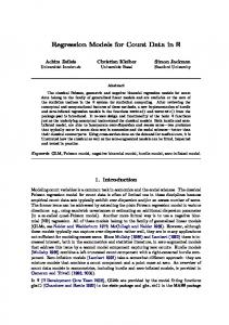
Fig. 1. Predicted Values of Mean Response and Standardized Deviance Residuals for Poisson and Negative Binomial Models Table 5 shows the regression parameters estimates for Multiple Negative Binomial Regression and Multiple Poisson Regression are somewhat similar. This is expected, as estimates from these models are consistent. Of the explanatory variables, the coefficient for the educational level of mother is negative and significant -0.144 and -0.173 for Multiple Negative Binomial Regression and Multiple Poisson Regression respectively which indicates that educated women have fewer children than uneducated women. As not expected, the coefficient for the dummy variable residence is positive indicating that there is no significant affect between rural and urban families. In summary, to some extent the estimation results support the neoclassical theory of fertility.

The standard errors of Negative Binomial Regression model are slightly higher than the standard errors of the Poisson model. Both models detected the appropriate sign for the relationship between fertility and wealth index and the coefficients for the fourth quintile and the richest quintile were statistically significant at 5% level of significance, indicating that fertility rate is higher among poor people compared to the rich. Multiple Poisson regression model also detected a significant difference in fertility rate between the poorest and second poorest quintiles.

Table 4. Bivariate Poisson regression verses multiple Poisson regression Variables Age of women Marital Status: Currently married=1 Formally married = 2 Never=3 Age at first marriage Years since first birth Partner/ husband has a wife: Yes=1 No=2 Currently using contraceptives: Yes=1 No=2

B 0.226

Bivariate Poisson regression P-value E (B) CI 0.00 1.253 1.245-1.261

Multiple Poisson regression B P-value E (B) C I 0.002 0.245 1.002 0.999-1.006

9.080 0.00 9.560 0.00 0 -0.046 0.00

8774.8 4388.2-17546.6 0 14188.6 7094.8-28375.2 1 0.955 0.952-0.958 -0.034

0.00

1 0.966 0.949 – 0.984

0.054

0.00

1.055

1.054-1.057

0.046

0.00

1.047 1.044- 1.051

0 -0.571 0.00

1 0.565

0.553-0.576

0 -0.019 0.123

1 0.957 – 1.005 0.981

0 0.91

1 1.095

1.060-1.131

0 -0.087 0.00

0.917 0.886 – 0.949

0.00

7

Ever had a child later died: Yes=1 No=2 Area: Rural Urban Highest educational level attained: University+ =5 Secondary =4 Intermediate=3 Primary=2 Khalwa=1 Illiterate = 0 Wealth Quintile: Richest: Fourth: Middle: Second: Poorest:

0.0 -0.572 0.00

0.565

0.536 - 0.94

0.0 -0.572 0.00

1 0.565 0.553 – 0.76

0.053 0.0

0.00

1.049 1

1.026-1.072

0.018 0.0

0.166

1.018 0.993 1.043

-0.60 -0.363 -0.076 -0.169 0.005 0

0.00 0.00 0.002 0.00 0.842

0.549 0.696 1.079 0.845 1.005 1

0.519-580 0.671-0.721 1.027-1.134 0.825-0.865 0.961-1.050

-0.173 -0.069 0.029 -0.014 0.017 0

0.00 0.002 0.295 0.326 0.418

0.841 0.933 1.029 0.987 1.018 1

0.784 - 0.902 0.893 – 0.975 0.975 – 1.086 0.960 – 1.014 0.976 – 1.061

-0.103 -0.049 -0.029 0.021 0

0.00 0.02 0.66 0.181

0.902 0.952 0.971 0.979 1

0.874-0.932 0.923-0.983 0.942-1.002 950-1.010

-0.143 -0.064 -0.025 -0.039 0

0.00 0.001 0.130 0.014

0.867 0.938 0.975 0.962 1

0.829 – 0.907 0.903 – 0.974 0.944 – 1.007 0.933 – 0.992

Table 5. Multiple Negative Binomial Regression and Multiple Poisson Regression Variables Age of women Marital Status: Currently married=1 Formally married =2 Never=3 Age at first marriage Years since first birth Partner/ husband has a wife: Yes=1 No=2 Currently using contraceptives: Yes=1 No=2 Ever had a child later died: Yes=1 No=2 Area: Rural= 2 Urban =1 Highest educational level attained: University+ =5 Secondary =4 Intermediate=3 Primary=2 Khalwa=1 Illiterate = 0 Wealth Quintile:

Multiple negative binomial regression B P-value E(B) CI 0.023 0.211 1.024 0.987 - 1.062

B 0.002

Multiple Poisson regression P-value E(B) C I 0.245 1.002 0.999-1.006

0 -0.044 0.054

0.035 0.00

1 0.957 1.055

0.919 - 0.997 1.047-1.063

0 -0.034 0.046

0 -0.018

0.555

1 0.982

0.982 – 1.044

0 -0.019 0.123

1 0.957 – 1.005 0.981

0 -0.088

0.034

1 0.916

0.845- 0.993

0 -0.087 0.00

1 0.917 0.886 – 0.949

0 -0.226

0.00

1 0.79

0.754 – 0.843

0 -0.232 0.00

0.793 0.776 – 0.811

0.00 0.00

1 0.966 1.047

0.949 – 0.984 1.044- 1.051

0.006 0

0.846

1.006 1

0.948 – 1.068

0.018 0.0

0.166

1.018 0.993 - 1.043

-0.144 -0.061 0.014 -0.014 0.007 0

0.052 0.228 0.844 0.672 0.899

0.866 0.941 1.014 0.986 1.007 1

0.749 – 1.001 0.853 – 1.039 0.886 – 1.160 0.925 – 1.052 0.906 – 1.119

-0.173 -0.069 0.029 -0.014 0.017 0.0

0.00 0.002 0.295 0.326 0.418

0.841 0.933 1.029 0.987 1.018 1

8

0.784 - 0.902 0.893 – 0.975 0.975 – 1.086 0.960 – 1.014 0.976 – 1.061

Richest: Fourth: Middle: Second: Poorest:

-0.154 -0.071 -0.038 -0.043 0.0

0.005 0.127 0.337 0.255

0.858 0.932 0.962 0.958 1

0.771 – 0.954 0.851 – 1.020 0.889 – 1.041 0.889 – 1.032

A negative and a highly significant relationship between fertility and age at first marriage is also is detected by the two models. This is supported by the theories and expectations because fertility span of those who get married at early ages, is longer and their chances in getting many children is higher.

-0.143 -0.064 -0.025 -0.039 0.0

0.00 0.001 0.130 0.014

0.867 0.938 0.975 0.962 1

0.829 – 0.907 0.903 – 0.974 0.944 – 1.007 0.933 – 0.992

COMPETING INTERESTS Authors have declared that no competing interests exist.

REFERENCE

Both of the two models have detected the appropriate relationship between child mortality and fertility, Those who ever had a child later died have higher fertility compared to those who had not, and this relationship is statistically significant. This supported by sense and logic as those who had a child later died try to compensate.

1.

2.

What worth noting is that, the multiple Poisson regression model has detected the correct relationship between using family planning and fertility whereas the negative regression model has not. Contrary to expectations, the negative regression model detected that fertility is higher among users of family planning methods compared to those who are not currently using family planning methods.

3.

4.

5. CONCLUSION This study demonstrates the performance of Negative binomial regression and the Generalized Poisson regression for explaining over dispersion count data. For comparing Negative Binomial Regression model and Poisson Regression model, we use two measures of goodness-of-fit like deviance and AIC for overdispersion. These values indicate that the Generalized Poisson Regression model is more appropriate for the present born data and leads to more efficient parameter estimates. Generalized Poisson Regression model detected the correct sign of relationship between dependent and independent variables whereas the negative binomial regression model failed to detect the correct relationship between currently using family planning methods and number of children ever born.

5.

6.

7.

8.

9.

That means, Generalized Poisson Regression model exhibits better explanation of child bearing which is a count data. Generalized Poisson Regression model shows that the population is growing at a very first rate in Sudan because of the effects of some typical demographic and socio-economic factors.

10.

11.

9

Al Awad. M. and Chartouni, C. Explaining the Decline in Fertility among Citizens of the G.C.C. Countries: the Case of the U.A.E. Institute for Social and Economic Research. 2014. Working Paper No. 1. Amarante. V. Determinants of Fertility at the Macro Level: New Evidence for Latin America and the Caribbean. 2014. The Journal of Developing Areas Volume 48.2. pp. 123-135. Bongaarts. John. Fertility and reproductive preferences in post-transitional societies. in Global Fertility Transition, Rodolfo A. Bulatao and John B. Casterline, eds. Population and Development Review Supplement to Vol. 27. New York, Population Council, pp. 260-281. 2001. Bongaarts. John. The fertility impact of changes in the timing of childbearing in the developing world. Population Studies 53:277289. 1999. Bongaarts. John. Trends in unwanted childbearing in the developing world. Studies in Family Planning 28(4):267-277. 1997a Bongaarts. John. The role of family planning programmes in contemporary fertility transitions. in the Continuing Demographic Transition. eds. Gavin W. Jones, Robert M. Douglas, John C. Caldwell, and Rennie M. D’Souza. Oxford: Clarendon Press, pp. 422– 443. 1997 Bongaarts. John. The impact of population policies: Comment. Population and Development Review 20(3): 616–620. 1994 Bongaarts. John. The KAP-gap and the unmet need for contraception. Population and Development Review 17(2): 293–313. 1991 Bongaarts. John and Griffith Feeney. On the quantum and tempo of fertility. Population and Development Review 24(2): 271-291.1988 Caldwell. J. C. Towards a restatement of demographic theory. Population and Development Review.1976. 2:321-366. Drèze, J. and Murthi, M. Fertility, Education, and Development: Evidence from India. 2001.

Population and Development Review.2013. 17. Kirk. D. and Pillet. B. Fertility levels, Trends 27: 33–63. and Differentials in Sub-Saharan Africa in the 12. Easterlin. R. A. and Eileen M. C. The Fertility 1980 and 1990s. 1998. Studies in Family Revolution: A Supply Demand Analysis. Planning, Volume 29 Number 1. University of Chicago Press Economic and 18. Long. J. S. Regression models for categorical Geographic Determinants Al Darah and limited dependent variables. 1997. Journal.1985. 28 (2): 9. 1999 Thousand Oaks, California: Sage Publications. 13. Eltigani. E. E. Understanding fertility decline 19. M. A. Khalifa. Determinates of natural fertility in Northern Sudan: an analysis of determinants. in Sudan. 1998. Journal of Biosocial Science. Genus. Università degli Studi di Roma. La 18. pp 325-336. Sapienza. Stable. 2000. Vol. 56, No. 1/2, pp. 20. Martin, T.C. and Juarez, F. The Impact of 115-132 Women's Education on Fertility in Latin 14. Hirschman. C. And Young. Yih-Jin. Social America: Searching for Explanations”. 1994. Context and Fertility Decline in Southeast International Family Planning Perspectives Asia: 1968-70 to 1988-90. 1994. Social Volume 21, Number 2. Context and Fertility Decline in Soul. 21. Sibanda, A., Woubalem, Z., Hogan, D. P. and 15. Hondroyiannis. G. Fertility Determinants and Lindstrom, D. P. The Proximate Determinants Economic Uncertainty: An Assessment Using of the Decline to Below-replacement Fertility European Panel Data. 2014. Working Papers in Addis. 2001 Ababa, Ethiopia. Studies in 96. Bank of Greece. Family Planning. 16. Khraif. R. Fertility in Saudi Arabia: Levels and 22. Vidal Zeballos. D. Social Strata and its Determinants. 2001. A paper presented at: influence on the Determinants of Reproductive XXIV. General Population Conference. Behavior in Bolivia. Macro International Inc. Salvador-Brazil, 18-24. 1994. Calverton, USA. __________________________________________________________________________________________ © Copyright International Knowledge Press. All rights reserved.

10