Using deep autoencoders to identify abnormal brain structural patterns in neuropsychiatric disorders: a large-scale multi-sample study Walter H. L. Pinaya * a b c, Andrea Mechelli c, João R. Sato a
* a Center of Mathematics, Computation, and Cognition. Universidade Federal do ABC, Santo André, Brazil. * b Center for Engineering, Modeling and Applied Social Sciences. Universidade Federal do ABC, Santo André, Brazil. c
Department of Psychosis Studies, Institute of Psychiatry, Psychology &
Neuroscience, King’s College London, London, UK.
* a Rua Arcturus, 03 - Jardim Antares, São Bernardo do Campo - SP, CEP 09.606-070, Brazil. * b Rua Arcturus, 03 - Jardim Antares, São Bernardo do Campo - SP, CEP 09.606-070, Brazil. c Institute
of Psychiatry, Psychology and Neuroscience, King’s College London,
De Crespigny Park, London SE5 8AF, UK.
Corresponding Author: Walter H. L. Pinaya Phone: +55 11 97123 0508 Email address:
[email protected]
1
Supplementary material Contents 1.
Information about the datasets ........................................................................................... 3
2.
MRI Acquisition..................................................................................................................... 5
3.
Performance of different deep autoencoder configurations ............................................... 6
4.
Comparison between deep autoencoder and linear method .............................................. 7
5.
Contribution of each input feature to the generation of the reconstructed data ............. 11
6.
Violin plot of the deviation metric ..................................................................................... 15
7.
Violin plot of reconstruction error of each region for the NUSDAST dataset .................... 16
8.
Violin plot of reconstruction error of each region for the ABIDE dataset .......................... 20
9.
Statistical significance and effect sizes of each region from the NUSDAST dataset .......... 24
10. Statistical significance and effect sizes of each region from the ABIDE dataset ................ 26 11. Mean original and reconstructed values of each region .................................................... 28 12. Mass-univariate analysis of the NUSDAST dataset ............................................................ 63 13. Mass-univariate analysis of the ABIDE dataset .................................................................. 65 14. Performance of the SVM classifiers.................................................................................... 67 References................................................................................................................................... 68
2
1. Information about the datasets
In this study, we used three datasets: the Human Connectome Project, the Northwestern University Schizophrenia Data and Software Tool (which is part of the Schizoconnect database), and the Autism Brain Imaging Data Exchange. Information about the three datastes is povided below.
Human Connectome Project The Human Connectome Project consortium led by Washington University, University of Minnesota, and Oxford University (the WU-Minn HCP consortium) is undertaking a systematic effort to characterize human brain connectivity and function in a large population of healthy adults [Van Essen et al., 2013]. The HCP aims to enable detailed comparisons between brain circuits, behavior, and genetics at the level of individual subjects. In this study, we use part of data from HCP database (https://db.humanconnectome.org).
Northwestern University Schizophrenia Data and Software Tool The NUSDAST database is a repository of schizophrenia neuroimaging data that shares sMRI data, genotyping data, and neurocognitive data as well as analysis tools to the schizophrenic research community. In this study, we use part of data from
NUSDAST
(http://central.xnat.org/REST/projects/NUDataSharing).
database As
such,
the
investigators within NUSDAST contributed to the design and implementation of
3
NUSDAST and/or provided data but did not participate in analysis or writing of this report.
SchizoConnect Project The SchizConnect project [Wang et al., 2016] is an initiative that allows combining of neuroimaging data from different databases via mediation to form compatible mega-datasets with high levels of accuracy and fidelity. The NUSDAST data used in
this
article
was
obtained
from
the
SchizConnect
database
(http://schizconnect.org). As such, the investigators within SchizConnect contributed to the design and implementation of SchizConnect and/or provided data but did not participate in analysis or writing of this report.
Autism Brain Imaging Data Exchange The Autism Brain Imaging Data Exchange (tinyurl.com/fcon1000-abide) started as an effort involving 17 international sites dedicated to aggregating and sharing previously collected data. This dataset is composed of resting state functional magnetic resonance imaging, anatomical and phenotypic datasets from individuals with autism spectrum disorder and age-matched typical controls [Di Martino et al., 2014].
4
2. MRI Acquisition
Human Connectome Project The HCP T1-weighted images were collected on a customized Siemens Skyra 3T scanner using a 32-channel head coil. Two separate averages of the T1w image are acquired using the 3D MPRAGE sequence with 0.7mm isotropic resolution (FOV=224 mm, matrix=320, 256 sagittal slices in a single slab), TR=2400 ms, TE=2.14 ms, flip angle =8°.
Northwestern University Schizophrenia Data and Software Tool The NUSDAST T1-weighted images were collected on a Siemens MAGNETOM VISION IMA. The neuroimages are acquired using 3D MPRAGE sequence TR=9.7 ms, TE=4 ms, flip=10°, ACQ=1, 256x256 matrix, 1 mm in-plane resolution, 128 slices, slice thickness 1.25 mm.
Autism Brain Imaging Data Exchange The ABIDE T1-weighted images were collected on multiple sites (twenty different sites in total). The acquisition parameters of each site are available at http://fcon_1000.projects.nitrc.org/indi/abide/abide_I.html.
5
3. Performance of different deep autoencoder configurations
Table 1 – Average reconstruction error of each tested configurations for the deep autoencoder. These values were obtained from the 10-fold cross-validation process performed using the data of the HCP dataset. The configuration chosen for further analyses is highlighted in bold. Details of the procedure followed to evaluate different neural network configuration is presented in Section “2.7 Performance evaluation of different network configurations” of the main document. Configuration
Reconstruction error Mean ± S.D.
25-10-25
0.610 ± 0.043
50-10-50
0.592 ± 0.029
75-10-75
0.580 ± 0.034
100-10-100
0.591 ±0.043
50-25-50
0.503 ±0.013
75-25-75
0.502 ± 0.017
100-25-100
0.540 ±0.101
75-50-75
0.441 ±0.011
100-50-100
0.482 ± 0.144
100-75-100
0.405 ±0.013
6
4. Comparison between deep autoencoder and linear method
In this study, we also performed the computation of the deviation metric using a well-known linear method, the Principal Components Analysis (PCA). Similar to the autoencoder, PCA is capable of performing (i) an encoding process where the input data are represented in the principal components space; and (ii) a decoding process where the representation is transformed back to the input space. Usually, PCA is used to perform dimensionality reduction tasks. This involves transforming the data into the principal components space (using the eigenvectors of the data covariance/correlation matrix). Following this transformation, only a part of the principal components dimensions – the ones that are responsible for explaining most of the variance in the input data (identified by the absolute value of the eigenvalues) - are used to represent the data. In order to compare the performance of PCA and that of the deep autoencoder, we followed the following procedure. First, we trained the PCA model to map the normalized input data to the principal components space using the whole HCP data. Next, we applied the learned transformation on each subject data from the clinical datasets. Then, we used a representation of the subjects’ data with reduced dimensionality (here we selected only the n principal components that are responsible for the most variance of the input data). Next, we transformed this reduced dimension representation back to the input space. Finally, we calculated the deviation metric using a similar approach to that used for the deep autoencoder (i.e. using the mean squared error between the input data and the reconstruction).
7
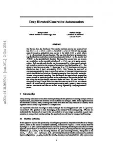
We defined the number of principal components used in the PCA based on the configuration of the deep autoencoder model with the smallest reconstruction error during the cross-validation. This model had 75 artificial neurons in its most abstract layer (the encoded representation); for this reason, when representing the input data into the principal components space, we used 75 dimensions to perform our comparison. The PCA method obtained a reconstruction error of 0.0355 for the HCP dataset. Figure 1 shows the explained variance of each principal component of the PCA method. Using 75 principal components, the data representation contains (or “explains”) 96.64% of the variance of the input data. The PCA obtained a deviation metric of 0.1183±0.0440 for the SCZ sample and a value of 0.1275±0.0369 for the HC sample of the NUSDAST dataset (p-value = 0.1453; Mann–Whitney U test). In the ABIDE balanced sample, the metric was 0.1241±0.0442 for the patients with ASD and 0.1430±0.0550 for the HC group (p-value = 0.0112; Mann–Whitney U test). For each dataset, we also computed the effect size of the difference between the patient and control groups using Cliff’s delta absolute value. The PCA method achieved an effect size of 0.1428 for the NUSDAST dataset (deep autoencoder’s effect size = 0.4142) and an effect size of 0.1940 for the ABIDE dataset (deep autoencoder’s effect size = 0.2764).
8
Figure 1 – Cumulative explained variance of the PCA model on the Human Connectome Project dataset. The vertical bars represent the individual explained variance of each principal component.
Therefore, in the analysis of disease-free subjects from the HCP dataset, the PCA approach achieved a smaller reconstruction error than the deep autoencoder. However, even with a better reconstruction error in disease-free subjects, the performance of the PCA approach was worse when it came to differentiating between the patient and control groups within each clinical dataset. In particular, while the PCA approach showed significantly different deviation metric values between the patient and control groups in the ABIDE dataset, it did not do so in the NUSDAST groups. Furthermore, for each clinical dataset, the PCA approach achieved a smaller effect size, indicating lower differentiation between the patient and control groups on the basis of their deviation metrics, than the deep autoencoder. These results might be explained by the capacity of the non-linear function that is incorporated in the deep autoencoder but not the PCA approach; alternatively, they might be explained by the inclusion of potential confounding variables (i.e., age and sex) in the deep autoencoder but not the 9
PCA approach. One limitation of this comparison is that the results are likely to be influenced by the choice of the number of principal components in the PCA model. In particular, the choice of a suboptimal hyperparameter can lead to a loss of information or the introduction of random noise. While there are a plethora of approaches for calculating the optimal number of principal components [Dray, 2008; Valle et al., 1999], none of them is universally recognised as the gold standard. The use of principal components equal to the number of neurons in the most abstract layer of the deep autoencoder might not be the most appropriate, however there is no standard approach to perform a comparison between these two methods.
10
5. Contribution of each input feature to the generation of the reconstructed data
One of the drawbacks of deep artificial neural networks is the difficulty of interpreting its internal computations. This lack of interpretability is the main reason why deep artificial networks are usually referred as “black box” models. In order to address this limitation, several studies have developed different methods Here we used one of these existing methods, known as guided backpropagation with SmoothGrad technique [Smilkov et al., 2017]. This method uses the network gradients to assign an “importance” value to individual elements of the autoencoder (in our case, the input features); this importance value is meant to reflect the influence of each element on the final loss function. Importance values are used to generate the so-called “saliency maps”. In particular, the SmoothGrad technique adds noise in the inputted data and generates the saliency map several times; this leads to the computation of an average saliency map which is thought to provide the most robust measure (for more technical details, see Smilkov et al., 2017). We used the above method to investigate the importance of each input feature (including the age and sex variables) to the generation of the reconstructed data. This allowed us to estimate the contribution of each brain region to the group classification decision, as well as the importance of each brain region for predicting the age and sex of the subjects. The interpretation of this method involved four main steps. First, we trained the deep autoencoder model using the whole normalized HCP dataset. Second, we used the trained model to generate the reconstructed values of each sample from the HCP dataset. Third,
11
using the guided backpropagation with SmoothGrad, we computed the network gradients based on the inputted data to generate the saliency map. Here the SmoothGrad technique was applied to 50 corrupted saliency maps in order to generate the final saliency map in each subject. Finally, we averaged the saliency map of all subjects within the same group to derive group-level saliency maps. A similar process was performed to determine the importance of the brain regions for predicting the age and sex. In this case the gradients were calculated based on their respective outputs loss function. Figure 2 and 3 show the mean saliency map of the reconstructed brain regions and the predicted age and sex.
Figure 2 – Mean saliency map of the reconstructed brain regions. The map was normalized to have values between 0 and 1. Each row of the saliency map represents an output unit of the deep autoencoder (i.e., a reconstructed brain region). The columns represent each input feature. The last two columns correspond to the influence of sex and age on the reconstruction of the brain regions.
12
Figure 3 - Mean saliency map of the predicted age and sex. The map was normalized to have values between 0 and 1. The columns represent each input feature.
Based on the mean salience maps, we were able to conclude that the model did not perform a trivial reconstruction of input feature or, in other words, it did not just copy the inputted data through the layers to generate the reconstructed data. This conclusion was based on the observation that the mean saliency map did not show an identity matrix pattern, where main diagonal has value 1 and all others elements have zero value. Instead, as shown in Figures 2 and 3, there was were diffused patterns in relation to the inputted data, especially in the case of cortical thickness. Figure 2 also shows that sex had relative high influence on the reconstruction of the volume of subcortical structures. The reason for the influence of sex on volumetric measures might be that the structural volumes of the subjects were not normalized by the total intracranial volume. The most influent regions for predicting sex were: optic chiasm volume, left amygdala volume, left cerebellum cortex volume, left temporal pole thickness, left caudate volume, 3rd ventricle volume, left superior frontal thickness, right superior temporal thickness, right putamen volume, left middle temporal 13
thickness, right lateral ventricle volume, right inferior lateral ventricle volume, left frontal pole thickness, left rostral middle frontal thickness, and left cerebellum cortex volume. In contrast, the most influent input features for predicting age were: left pallidum volume, brain stem volume, anterior corpus callosum volume, optic chiasm volume, right hippocampus volume, right caudal middle frontal thickness, left rostral anterior cingulate thickness, right pallidum volume, posterior corpus callosum, right precuneus thickness, left insula thickness, left caudal middle frontal thickness right putamen volume, right entorhinal thickness, and left caudal anterior cingulate thickness.
14
6. Violin plot of the deviation metric
Figure 4 - Violin plot of the deviation metric of each group of each dataset. The median and the Interquartile range are presented.
15
7. Violin plot of reconstruction error of each region for the NUSDAST dataset
16
Continuation of violin plot of reconstruction error of each region for the NUSDAST dataset
17
Continuation of violin plot of reconstruction error of each region for the NUSDAST dataset
18
Continuation of violin plot of reconstruction error of each region for the NUSDAST dataset
Figure 5 - Violin plot of the reconstruction error of each brain regions analyzed by the deep autoencoder using the NUSDAST dataset. The medians of the distributions are indicated by the red line.
19
8. Violin plot of reconstruction error of each region for the ABIDE dataset
20
Continuation of violin plot of reconstruction error of each region for the ABIDE dataset
21
Continuation of violin plot of reconstruction error of each region for the ABIDE dataset
22
Continuation of violin plot of reconstruction error of each region for the ABIDE dataset
Figure 6 - Violin plot of the reconstruction error of each brain regions analyzed by the deep autoencoder using the ABIDE dataset. The medians of the distributions are indicated by the red line.
23
9. Statistical significance and effect sizes of each region from the NUSDAST dataset Table 2 - Statistical significance measured by the Mann-Whitney U test and effect size measured by Cliff’s delta absolute value based on the comparison of the reconstruction error of each brain of the groups from NUSDAST dataset. The significant regions (alpha >= 0.01) are highlighted in bold. p-value
Effect size
Regions
p-value
Effect size
Left-Lateral-Ventricle
.0011
.4100
lh_parsopercularis
.4472
.0185
Left-Inf-Lat-Vent
.2302
.1000
lh_parsorbitalis
.1502
.1400
Left-Cerebellum-White-Matter
.0276
.2585
lh_parstriangularis
.4640
.0128
Left-Cerebellum-Cortex
.1080
.1671
lh_pericalcarine
.1358
.1485
Left-Thalamus-Proper
.0256
.2628
lh_postcentral
.1603
.1342
Left-Caudate
.1876
.1200
lh_posteriorcingulate
.3413
.0557
Left-Putamen
.4014
.0342
lh_precentral
.0090
.3185
Left-Pallidum
.0515
.2200
lh_precuneus
.0403
.2357
3rd-Ventricle
.0334
.2471
lh_rostralanteriorcingulate
.0637
.2057
4th-Ventricle
.2958
.0728
lh_rostralmiddlefrontal
.1552
.1371
Brain-Stem
.0161
.2885
lh_superiorfrontal
.4014
.0342
Left-Hippocampus
.2849
.0771
lh_superiorparietal
.0966
.1757
Left-Amygdala
.2400
.0957
lh_superiortemporal
.1181
.1600
CSF
.2778
.0800
lh_supramarginal
.3730
.0442
Left-Accumbens-area
.0104
.3114
lh_frontalpole
.3297
.0600
Left-VentralDC
.0009
.4171
lh_temporalpole
.3891
.0385
Left-choroid-plexus
.4640
.0128
lh_transversetemporal
.3374
.0571
Right-Lateral-Ventricle
.0074
.3285
lh_insula
.0765
.1928
Right-Inf-Lat-Vent
.1763
.1257
rh_bankssts
.1290
.1528
Right-Cerebellum-White-Matter
.1003
.1728
rh_caudalanteriorcingulate
.4767
.0085
Right-Cerebellum-Cortex
.0226
.2700
rh_caudalmiddlefrontal
.0515
.2200
Right-Thalamus-Proper
.1429
.1442
rh_cuneus
.4388
.0214
Right-Caudate
.0549
.2157
rh_entorhinal
.2672
.0842
Right-Putamen
.1763
.1257
rh_fusiform
.1429
.1442
Right-Pallidum
.0157
.2900
rh_inferiorparietal
.4097
.0314
Right-Hippocampus
.1060
.1685
rh_inferiortemporal
.1290
.1528
Right-Amygdala
.3452
.0542
rh_isthmuscingulate
.1453
.1428
Right-Accumbens-area
.2707
.0828
rh_lateraloccipital
.2433
.0942
Right-VentralDC
.0130
.3000
rh_lateralorbitofrontal
.0692
.2000
Right-choroid-plexus
.0561
.2142
rh_lingual
.3452
.0542
Optic-Chiasm
.2144
.1071
rh_medialorbitofrontal
.0765
.1928
CC_Posterior
.0403
.2357
rh_middletemporal
.2602
.0871
CC_Mid_Posterior
.3182
.0642
rh_parahippocampal
.4514
.0171
Regions
24
CC_Central
.4388
.0214
rh_paracentral
.0948
.1771
CC_Mid_Anterior
.3689
.0457
rh_parsopercularis
.0845
.1857
CC_Anterior
.0895
.1814
rh_parsorbitalis
.3144
.0657
lh_bankssts
.2534
.0900
rh_parstriangularis
.3810
.0414
lh_caudalanteriorcingulate
.4472
.0185
rh_pericalcarine
.2534
.0900
lh_caudalmiddlefrontal
.2144
.1071
rh_postcentral
.1763
.1257
lh_cuneus
.1682
.1300
rh_posteriorcingulate
.0412
.2342
lh_entorhinal
.2602
.0871
rh_precentral
.3610
.0485
lh_fusiform
.1904
.1185
rh_precuneus
.2742
.0814
lh_inferiorparietal
.4851
.0057
rh_rostralanteriorcingulate
.2958
.0728
lh_inferiortemporal
.2885
.0757
rh_rostralmiddlefrontal
.1629
.1328
lh_isthmuscingulate
.0130
.3000
rh_superiorfrontal
.3491
.0528
lh_lateraloccipital
.1876
.1200
rh_superiorparietal
.4138
.0300
lh_lateralorbitofrontal
.1060
.1685
rh_superiortemporal
.0020
.3871
lh_lingual
.1791
.1242
rh_supramarginal
.4978
.0014
lh_medialorbitofrontal
.1080
.1671
rh_frontalpole
.4014
.0342
lh_middletemporal
.1992
.1142
rh_temporalpole
.3491
.0528
lh_parahippocampal
.0504
.2214
rh_transversetemporal
.3069
.0685
lh_paracentral
.3891
.0385
rh_insula
.4556
.0157
25
10.
Statistical significance and effect sizes of each region from
the ABIDE dataset Table 3 - Statistical significance measured by the Mann-Whitney U test and effect size measured by Cliff’s delta absolute value based on the comparison of the reconstruction error of each brain of the groups from ABIDE dataset. The significant regions (alpha >= 0.01) are highlighted in bold. p-value
Effect size
Regions
p-value
Effect size
Left-Lateral-Ventricle
.2145
0674
lh_parsopercularis
.4166
.0180
Left-Inf-Lat-Vent
.1636
.0834
lh_parsorbitalis
.3812
.0258
Left-Cerebellum-White-Matter
.0886
.1149
lh_parstriangularis
.1822
.0772
Left-Cerebellum-Cortex
.0046
.2216
lh_pericalcarine
.3699
.0283
Left-Thalamus-Proper
.4731
.0059
lh_postcentral
.2603
.0547
Left-Caudate
.0990
.1096
lh_posteriorcingulate
.1072
.1057
Left-Putamen
.0037
.2280
lh_precentral
.3988
.0219
Left-Pallidum
.0957
.1112
lh_precuneus
.2559
.0559
3rd-Ventricle
.1475
.0892
lh_rostralanteriorcingulate
.0217
.1718
4th-Ventricle
.4957
.0010
lh_rostralmiddlefrontal
.2799
.0497
Brain-Stem
.3802
.0260
lh_superiorfrontal
.1773
.0788
Left-Hippocampus
.2021
.0710
lh_superiorparietal
.1649
.0830
Left-Amygdala
.1438
.0905
lh_superiortemporal
.3478
.0334
CSF
.3078
.0428
lh_supramarginal
.3578
.0311
Left-Accumbens-area
.1378
.0928
lh_frontalpole
.4082
.0199
Left-VentralDC
.1724
.0804
lh_temporalpole
.1738
.0800
Left-choroid-plexus
.0017
.2496
lh_transversetemporal
.3300
.0375
Right-Lateral-Ventricle
.0966
.1107
lh_insula
.3792
.0263
Right-Inf-Lat-Vent
.1801
.0779
rh_bankssts
.2533
.0566
Right-Cerebellum-White-Matter
.3203
.0398
rh_caudalanteriorcingulate
.1551
.0864
Right-Cerebellum-Cortex
.1710
.0809
rh_caudalmiddlefrontal
.3222
.0394
Right-Thalamus-Proper
.0547
.1362
rh_cuneus
.0020
.2448
Right-Caudate
.2241
.0646
rh_entorhinal
.1164
.1015
Right-Putamen
.0180
.1784
rh_fusiform
.4817
.0040
Right-Pallidum
.2456
.0586
rh_inferiorparietal
.2542
.0563
Right-Hippocampus
.2551
.0561
rh_inferiortemporal
.1643
.0832
Right-Amygdala
.0222
.1711
rh_isthmuscingulate
.4699
.0065
Right-Accumbens-area
.3021
.0442
rh_lateraloccipital
.0104
.1966
Right-VentralDC
.0688
.1263
rh_lateralorbitofrontal
.2700
.0522
Right-choroid-plexus
.1360
.0935
rh_lingual
.1703
.0811
Optic-Chiasm
.3999
.0217
rh_medialorbitofrontal
.2718
.0517
CC_Posterior
.3003
.0446
rh_middletemporal
.4072
.0201
Regions
26
CC_Mid_Posterior
.4527
.0102
rh_parahippocampal
.3967
.0224
CC_Central
.1616
.0841
rh_paracentral
.0740
.1231
CC_Mid_Anterior
.1513
.0878
rh_parsopercularis
.0217
.1718
CC_Anterior
.2298
.0630
rh_parsorbitalis
.3174
.0405
lh_bankssts
.3528
.0322
rh_parstriangularis
.3628
.0299
lh_caudalanteriorcingulate
.0613
.1314
rh_pericalcarine
.4527
.0102
lh_caudalmiddlefrontal
.2709
.0520
rh_postcentral
.3040
.0437
lh_cuneus
.1251
.0979
rh_posteriorcingulate
.2674
.0529
lh_entorhinal
.0562
.1351
rh_precentral
.4357
.0139
lh_fusiform
.1112
.1038
rh_precuneus
.0445
.1447
lh_inferiorparietal
.3031
.0439
rh_rostralanteriorcingulate
.4517
.0104
lh_inferiortemporal
.2098
.0687
rh_rostralmiddlefrontal
.1939
.0736
lh_isthmuscingulate
.4613
.0084
rh_superiorfrontal
.4314
.0148
lh_lateraloccipital
.3853
.0249
rh_superiorparietal
.3031
.0439
lh_lateralorbitofrontal
.3116
.0419
rh_superiortemporal
.2665
.0531
lh_lingual
.4860
.0031
rh_supramarginal
.1290
.0963
lh_medialorbitofrontal
.1112
.1038
rh_frontalpole
.4817
.0040
lh_middletemporal
.4806
.0042
rh_temporalpole
.2612
.0545
lh_parahippocampal
.3164
.0407
rh_transversetemporal
.0227
.1702
lh_paracentral
.2937
.0462
rh_insula
.3874
.0244
27
11.
Mean original and reconstructed values of each region
Here, for each dataset, we reported the mean original and reconstructed values in each brain region and in each group, with the error bars representing the standard deviation. For each dataset, the healthy control group is shown in black and the patient group is shown in red. A dashed horizontal line is used to help compare the original and reconstructed values. The original values were normalized using the Human Connectome Project statistics (mean and standard deviation).
28
29
30
31
32
33
34
35
36
37
38
39
40
41
42
43
44
45
46
47
48
49
50
51
52
53
54
55
56
57
58
59
60
61
62
12.
Mass-univariate analysis of the NUSDAST dataset
Table 4 – Mass univariate analysis of the NUSDAST dataset performed using Mann-Whitney U test and effect size measured by Cliff’s delta value based on the original thickness and volume of each brain region. The significant regions (alpha >= 0.01) are highlighted in bold. Negative values indicate higher values on the patient group. p-value
Effect size
Regions
p-value
Effect size
Left-Lateral-Ventricle
.3491
0.0529
lh_parsopercularis
.0879
0.1829
Left-Inf-Lat-Vent
.0829
-0.1871
lh_parsorbitalis
.3336
0.0586
Left-Cerebellum-White-Matter
.0210
0.2743
lh_parstriangularis
.3933
0.0371
Left-Cerebellum-Cortex
.1041
0.1700
lh_pericalcarine
.3014
0.0707
Left-Thalamus-Proper
.0171
0.2857
lh_postcentral
.0472
0.2257
Left-Caudate
.2335
-0.0986
lh_posteriorcingulate
.4056
0.0329
Left-Putamen
.0483
-0.2243
lh_precentral
.0091
0.3186
Left-Pallidum
.0002
-0.4786
lh_precuneus
.0605
0.2093
3rd-Ventricle
.0082
-0.3236
lh_rostralanteriorcingulate
.3491
-0.0529
4th-Ventricle
.2534
0.0900
lh_rostralmiddlefrontal
.4451
0.0193
Brain-Stem
.1041
0.1700
lh_superiorfrontal
.0829
0.1871
Left-Hippocampus
.1683
0.1300
lh_superiorparietal
.0556
0.2150
Left-Amygdala
.2534
0.0900
lh_superiortemporal
.0273
0.2593
CSF
.2672
-0.0843
lh_supramarginal
.0372
0.2407
Left-Accumbens-area
.1290
0.1529
lh_frontalpole
.2832
0.0779
Left-VentralDC
.1358
0.1486
lh_temporalpole
.4788
0.0079
Left-choroid-plexus
.4180
0.0286
lh_transversetemporal
.0521
0.2193
Right-Lateral-Ventricle
.3650
0.0471
lh_insula
.0097
0.3150
Right-Inf-Lat-Vent
.1552
-0.1371
rh_bankssts
.0012
0.4100
Right-Cerebellum-White-Matter
.0127
0.3014
rh_caudalanteriorcingulate
.0813
0.1886
Right-Cerebellum-Cortex
.0813
0.1886
rh_caudalmiddlefrontal
.0339
0.2464
Right-Thalamus-Proper
.0781
0.1914
rh_cuneus
.1833
0.1221
Right-Caudate
.1502
-0.1400
rh_entorhinal
.2083
0.1100
Right-Putamen
.0114
-0.3071
rh_fusiform
.0205
0.2757
Right-Pallidum
.0018
-0.3914
rh_inferiorparietal
.0103
0.3121
Right-Hippocampus
.2238
0.1029
rh_inferiortemporal
.0390
0.2379
Right-Amygdala
.2367
0.0971
rh_isthmuscingulate
.3892
-0.0386
Right-Accumbens-area
.4097
0.0314
rh_lateraloccipital
.0009
0.4221
Right-VentralDC
.3374
0.0571
rh_lateralorbitofrontal
.1013
0.1721
Right-choroid-plexus
.2832
-0.0779
rh_lingual
.0658
0.2036
Optic-Chiasm
.2977
-0.0721
rh_medialorbitofrontal
.0751
0.1943
CC_Posterior
.0665
0.2029
rh_middletemporal
.0638
0.2057
CC_Mid_Posterior
.0611
0.2086
rh_parahippocampal
.1478
0.1414
Regions
63
CC_Central
.3221
0.0629
rh_paracentral
.0957
0.1764
CC_Mid_Anterior
.2052
0.1114
rh_parsopercularis
.0948
0.1771
CC_Anterior
.4979
0.0000
rh_parsorbitalis
.1301
0.1521
lh_bankssts
.0403
0.2357
rh_parstriangularis
.2191
0.1050
lh_caudalanteriorcingulate
.4514
0.0171
rh_pericalcarine
.3912
0.0379
lh_caudalmiddlefrontal
.1527
0.1386
rh_postcentral
.0032
0.3671
lh_cuneus
.0499
0.2221
rh_posteriorcingulate
.2450
0.0936
lh_entorhinal
.1100
0.1657
rh_precentral
.0093
0.3171
lh_fusiform
.0477
0.2250
rh_precuneus
.0351
0.2443
lh_inferiorparietal
.0129
0.3007
rh_rostralanteriorcingulate
.1130
0.1636
lh_inferiortemporal
.0093
0.3171
rh_rostralmiddlefrontal
.2254
0.1021
lh_isthmuscingulate
.4242
0.0264
rh_superiorfrontal
.0462
0.2271
lh_lateraloccipital
.0027
0.3750
rh_superiorparietal
.0112
0.3079
lh_lateralorbitofrontal
.0359
0.2429
rh_superiortemporal
.0287
0.2564
lh_lingual
.0343
0.2457
rh_supramarginal
.0109
0.3093
lh_medialorbitofrontal
.4619
0.0136
rh_frontalpole
.2400
0.0957
lh_middletemporal
.4118
0.0307
rh_temporalpole
.4263
0.0257
lh_parahippocampal
.0446
0.2293
rh_transversetemporal
.0158
0.2900
lh_paracentral
.0624
0.2071
rh_insula
.2160
0.1064
64
13.
Mass-univariate analysis of the ABIDE dataset
Table 5 - Mass univariate analysis of the ABIDE dataset performed using Mann-Whitney U test and effect size measured by Cliff’s delta value based on the original thickness and volume of each brain region. The significant regions (alpha >= 0.01) are highlighted in bold. Negative values indicate higher values on the patient group. p-value
Effect size
Regions
p-value
Effect size
Left-Lateral-Ventricle
.0630
-0.1302
lh_parsopercularis
.4367
0.0137
Left-Inf-Lat-Vent Left-Cerebellum-WhiteMatter Left-Cerebellum-Cortex
.0002
-0.3020
lh_parsorbitalis
.3059
0.0433
.4688
-0.0068
lh_parstriangularis
.0862
0.1161
.1279
0.0967
lh_pericalcarine
.4314
0.0148
Left-Thalamus-Proper
.3116
-0.0419
lh_postcentral
.0608
0.1317
Left-Caudate
.4860
-0.0031
lh_posteriorcingulate
.3398
0.0352
Left-Putamen
.1776
-0.0787
lh_precentral
.4871
0.0029
Left-Pallidum
.3212
-0.0396
lh_precuneus
.0370
0.1520
3rd-Ventricle
.0912
-0.1135
lh_rostralanteriorcingulate
.1557
0.0862
4th-Ventricle
.2809
0.0495
lh_rostralmiddlefrontal
.2067
0.0697
Brain-Stem
.2577
0.0554
lh_superiorfrontal
.4463
0.0116
Left-Hippocampus
.1481
-0.0889
lh_superiorparietal
.0610
0.1316
Left-Amygdala
.0969
-0.1106
lh_superiortemporal
.4108
-0.0193
CSF
.3232
-0.0391
lh_supramarginal
.2660
0.0532
Left-Accumbens-area
.2683
-0.0527
lh_frontalpole
.3126
0.0417
Left-VentralDC
.0600
-0.1323
lh_temporalpole
.3543
-0.0319
Left-choroid-plexus
.2025
0.0709
lh_transversetemporal
.1522
-0.0874
Right-Lateral-Ventricle
.4892
0.0024
lh_insula
.0608
0.1317
Right-Inf-Lat-Vent Right-Cerebellum-WhiteMatter Right-Cerebellum-Cortex
.0157
-0.1830
rh_bankssts
.3638
0.0297
.3822
-0.0256
rh_caudalanteriorcingulate
.0681
0.1268
.3339
0.0366
rh_caudalmiddlefrontal
.2298
0.0630
Right-Thalamus-Proper
.3092
0.0425
rh_cuneus
.0215
0.1721
Right-Caudate
.4346
0.0141
rh_entorhinal
.4887
-0.0025
Right-Putamen
.4293
-0.0153
rh_fusiform
.4272
0.0157
Right-Pallidum
.3623
-0.0301
rh_inferiorparietal
.0449
0.1443
Right-Hippocampus
.0322
-0.1573
rh_inferiortemporal
.3300
0.0375
Right-Amygdala
.1123
-0.1034
rh_isthmuscingulate
.0774
0.1211
Right-Accumbens-area
.4193
-0.0174
rh_lateraloccipital
.2499
0.0575
Right-VentralDC
.1942
-0.0734
rh_lateralorbitofrontal
.0414
0.1476
Right-choroid-plexus
.2951
0.0459
rh_lingual
.1920
0.0741
Optic-Chiasm
.2322
-0.0623
rh_medialorbitofrontal
.0812
0.1189
CC_Posterior
.0332
0.1562
rh_middletemporal
.1762
0.0792
Regions
65
CC_Mid_Posterior
.3373
0.0358
rh_parahippocampal
.0903
0.1139
CC_Central
.4219
0.0169
rh_paracentral
.0757
0.1221
CC_Mid_Anterior
.4618
0.0083
rh_parsopercularis
.1738
0.0800
CC_Anterior
.0213
0.1725
rh_parsorbitalis
.0135
0.1881
lh_bankssts
.1593
0.0849
rh_parstriangularis
.1115
0.1037
lh_caudalanteriorcingulate
.0966
0.1107
rh_pericalcarine
.3433
0.0344
lh_caudalmiddlefrontal
.4469
-0.0115
rh_postcentral
.1928
0.0739
lh_cuneus
.1077
0.1055
rh_posteriorcingulate
.2205
0.0656
lh_entorhinal
.3931
-0.0232
rh_precentral
.2410
0.0599
lh_fusiform
.1797
0.0780
rh_precuneus
.0036
0.2289
lh_inferiorparietal
.0205
0.1738
rh_rostralanteriorcingulate
.1042
0.1071
lh_inferiortemporal
.4293
-0.0153
rh_rostralmiddlefrontal
.1194
0.1003
lh_isthmuscingulate
.1128
0.1032
rh_superiorfrontal
.2905
0.0470
lh_lateraloccipital
.0289
0.1614
rh_superiorparietal
.0786
0.1204
lh_lateralorbitofrontal
.0888
0.1147
rh_superiortemporal
.2478
0.0581
lh_lingual
.4667
0.0072
rh_supramarginal
.1348
0.0940
lh_medialorbitofrontal
.4298
0.0151
rh_frontalpole
.2397
0.0602
lh_middletemporal
.2129
0.0678
rh_temporalpole
.4415
-0.0126
lh_parahippocampal
.1351
0.0939
rh_transversetemporal
.0990
0.1096
lh_paracentral
.3275
0.0381
rh_insula
.0463
0.1431
66
14.
Performance of the SVM classifiers
Table 6 - Performance of the linear SVM classifiers in the NUSDAST and ABIDE datasets. These performances were obtain using a bootstrap resampling method using 10,000 repetitions. These metrics were obtained in the task of classification between healthy controls and patients.
Balance accuracy
Sensitivity
Specificity
Error rate
NUSDAST
.588 [.462, .766]
.529 [.222, .824]
.650 [.400, .875]
.415 [.282, .543]
ABIDE
.552 [.460, .63]
.476 [.308, .659]
.621 [.453, .778]
.443 [.352, .535]
Dataset
*Values presented as median estimate [95% confidence interval].
67
References
Dray S (2008): On the number of principal components: A test of dimensionality based on measurements of similarity between matrices. Comput Stat Data Anal 52:2228–2237. Van Essen DC, Smith SM, Barch DM, Behrens TEJ, Yacoub E, Ugurbil K (2013): The WU-Minn Human Connectome Project: An overview. Neuroimage 80:62–79. http://dx.doi.org/10.1016/j.neuroimage.2013.05.041. Grün F, Rupprecht C, Navab N, Tombari F (2016): A Taxonomy and Library for Visualizing Learned Features in Convolutional Neural Networks. arXiv Prepr arXiv160607757. Di Martino A, Yan C-G, Li Q, Denio E, Castellanos FX, Alaerts K, Anderson JS, Assaf M, Bookheimer SY, Dapretto M (2014): The autism brain imaging data exchange: towards a large-scale evaluation of the intrinsic brain architecture in autism. Mol Psychiatry 19:659–667. Milham MP, Fair D, Mennes M, Mostofsky SHMD (2012): The ADHD-200 consortium: a model to advance the translational potential of neuroimaging in clinical neuroscience. Front Syst Neurosci 6:62. Selvaraju RR, Das A, Vedantam R, Cogswell M, Parikh D, Batra D (2016): Grad-cam: Why did you say that? visual explanations from deep networks via gradient-based localization. arXiv Prepr arXiv161002391. Smilkov D, Thorat N, Kim B, Viégas F, Wattenberg M (2017): SmoothGrad: removing noise by adding noise. arXiv Prepr arXiv170603825. Springenberg JT, Dosovitskiy A, Brox T, Riedmiller M (2014): Striving for simplicity: The all convolutional net. arXiv Prepr arXiv14126806. Valle S, Li W, Qin SJ (1999): Selection of the number of principal components: the variance of the reconstruction error criterion with a comparison to other methods. Ind Eng Chem Res 38:4389–4401. Wang L, Alpert KI, Calhoun VD, Cobia DJ, Keator DB, King MD, Kogan A, Landis D, Tallis M, Turner MD, Potkin SG, Turner JA, Ambite JL (2016): SchizConnect: Mediating neuroimaging databases on schizophrenia and related disorders for large-scale integration. Neuroimage 124:1155–1167. http://dx.doi.org/10.1016/j.neuroimage.2015.06.065.
68