Such denoising autoencoders are stacked and trained to initialize a deep neural ... an information theoretic perspective or a generative model perspective.
Category: Learning algorithms
Preference: oral
1
Deep Learning with Denoising Autoencoders Pascal Vincent, Hugo Larochelle, Yoshua Bengio and Pierre-Antoine Manzagol Dept. IRO, Universit´e de Montr´eal, C.P. 6128, Montreal, Qc, H3C 3J7, Canada {vincentp,larocheh,bengioy,manzagop}@iro.umontreal.ca http://www.iro.umontreal.ca/∼lisa Previous work has shown that the difficulties in learning deep generative or discriminative models can be overcome by an initial unsupervised learning step that maps inputs to useful intermediate representations (Hinton et al., 2006; Hinton & Salakhutdinov, 2006; Bengio et al., 2007; Ranzato et al., 2007; Larochelle et al., 2007; Lee et al., 2008). While unsupervised learning of a mapping that produces “good” intermediate representations of the input pattern seems to be key, little is understood regarding what constitutes “good” representations for initializing deep architectures, or what criteria may guide learning such representations. Here we hypothesize and investigate a specific criterion: robustness to partial destruction of the input. In Bengio et al. (2007), basic autoencoders have been used as a building block to initialize deep networks. Here we propose to use instead denoising autoencoders, which are trained to reconstruct a clean “repaired” input from a corrupted, partially destroyed one (see figure 1 for a schematic representation of the process). Such denoising autoencoders are stacked and trained to initialize a deep neural network, which is then globally fine tuned using a supervised criterion. The algorithm can be motivated from a manifold learning perspective an information theoretic perspective or a generative model perspective. Experiments clearly show the surprising advantage of corrupting the input of autoencoders on a pattern classification benchmark suite (see table 1 and figure 2). y fθ
˜ x
gθ0 qD
x
˜ . The autoencoder then maps it to y and attempts to reconstruct x. Figure 1: An example x is corrupted to x
Table 1: Comparison of stacked denoising autoencoders (SdA-3) with SVMs and Deep Belief Nets Test error rate on all considered classification problems is reported together with a 95% confidence interval. Best performer is in bold, as well as those for which confidence intervals overlap. SdA-3 appears to achieve performance superior or equivalent to the best other model on all problems except bg-rand. For SdA-3, we also indicate the fraction ν of destroyed input components, as chosen by proper model selection. Note that SAA-3 is equivalent to SdA-3 with ν = 0%. Dataset basic rot bg-rand bg-img rot-bg-img rect rect-img convex
SVMrbf 3.03±0.15 11.11±0.28 14.58±0.31 22.61±0.37 55.18±0.44 2.15±0.13 24.04±0.37 19.13±0.34
SVMpoly 3.69±0.17 15.42±0.32 16.62±0.33 24.01±0.37 56.41±0.43 2.15±0.13 24.05±0.37 19.82±0.35
DBN-1 3.94±0.17 14.69±0.31 9.80±0.26 16.15±0.32 52.21±0.44 4.71±0.19 23.69±0.37 19.92±0.35
SAA-3 3.46±0.16 10.30±0.27 11.28±0.28 23.00±0.37 51.93±0.44 2.41±0.13 24.05±0.37 18.41±0.34
DBN-3 3.11±0.15 10.30±0.27 6.73±0.22 16.31±0.32 47.39±0.44 2.60±0.14 22.50±0.37 18.63±0.34
SdA-3 (ν) 2.80±0.14 (10%) 10.29±0.27 (10%) 10.38±0.27 (40%) 16.68±0.33 (25%) 44.49±0.44 (25%) 1.99±0.12 (10%) 21.59±0.36 (25%) 19.06±0.34 (10%)
(a) No destroyed inputs
(b) 25% destruction
(d) Neuron A (0%, 10%, 20%, 50% destruction)
(c) 50% destruction
(e) Neuron B (0%, 10%, 20%, 50% destruction)
Figure 2: Filters obtained after training the first denoising autoencoder. (a-c) show some of the filters obtained after training a denoising autoencoder on MNIST samples, with increasing destruction levels ν. The filters at the same position in the three images are related only by the fact that the autoencoders were started from the same random initialization point. (d) and (e) zoom in on the filters obtained for two of the neurons, again for increasing destruction levels. As can be seen, with no noise, many filters remain similarly uninteresting (undistinctive almost uniform grey patches). As we increase the noise level, denoising training forces the filters to differentiate more, and capture more distinctive features. Higher noise levels tend to induce less local filters, as expected. One can distinguish different kinds of filters, from local blob detectors, to stroke detectors, and some full character detectors at the higher noise levels.
References Bengio, Y., Lamblin, P., Popovici, D., & Larochelle, H. (2007). Greedy layer-wise training of deep networks. Advances in Neural Information Processing Systems 19 (pp. 153–160). MIT Press. Hinton, G., & Salakhutdinov, R. (2006). Reducing the dimensionality of data with neural networks. Science, 313, 504–507. Hinton, G. E., Osindero, S., & Teh, Y. (2006). A fast learning algorithm for deep belief nets. Neural Computation, 18, 1527–1554. Larochelle, H., Erhan, D., Courville, A., Bergstra, J., & Bengio, Y. (2007). An empirical evaluation of deep architectures on problems with many factors of variation. Twenty-fourth International Conference on Machine Learning (ICML’2007). Lee, H., Ekanadham, C., & Ng, A. (2008). Sparse deep belief net model for visual area V2. In J. Platt, D. Koller, Y. Singer and S. Roweis (Eds.), Advances in neural information processing systems 20. Cambridge, MA: MIT Press. Ranzato, M., Poultney, C., Chopra, S., & LeCun, Y. (2007). Efficient learning of sparse representations with an energy-based model. Advances in Neural Information Processing Systems (NIPS 2006). MIT Press.
2