Using durational cues in a computational model of spoken-word

Using durational cues in a computational model of spoken-word recognition Odette Scharenborg Centre for Language and Speech Technology, Radboud University Nijmegen, The Netherlands [email protected]

Abstract Evidence that listeners use durational cues to help resolve temporarily ambiguous speech input has accumulated over the past few years. In this paper, we investigate whether durational cues are also beneficial for word recognition in a computational model of spoken-word recognition. Two sets of simulations were carried out using the acoustic signal as input. The simulations showed that the computational model, like humans, takes benefit from durational cues during word recognition, and uses these to disambiguate the speech signal. These results thus provide support for the theory that durational cues play a role in spoken-word recognition. Index Terms: duration, spoken-word recognition, computational modelling

1. Introduction Evidence that listeners (at least in a laboratory environment) use durational cues to help resolve temporarily ambiguous speech input has accumulated over the past few years (e.g., [13]). In order for any computational model of spoken-word recognition to be able to account for these data, it should be able to extract durational cues from the acoustic signal and use these during word recognition. In [4], we presented a novel computational model of spoken-word recognition designed for ‘tracking’ subtle phonetic information in the acoustic speech signal and using it during word recognition: Fine-Tracker. The first modelling results with Fine-Tracker were promising: an initial simulation using the acoustic material from the behavioural study presented in [2] showed that, like listeners, Fine-Tracker can distinguish short words (e.g., ‘ham’) from the longer words in which they are embedded (e.g., ‘hamster’). In this paper, we further investigate whether durational information is beneficial for Fine-Tracker in two sets of simulations. In the first simulation, Fine-Tracker is tested on its ability to distinguish monosyllabic words from the longer words in which they are embedded. This simulation is a replication and an extension of the work presented in [4]. We investigate the effect of duration by testing Fine-Tracker in two conditions: with and without the ability to use the duration cues in the speech signal. The second simulation focuses on the differences in durations of a single segment.

2. Fine-Tracker Fine-Tracker [4] is based on the theory underlying Shortlist [5], which holds that the speech recognition process consists of two levels. First, listeners map the incoming acoustic signal onto so-called prelexical representations at the prelexical level. At the lexical level, all representations are stored in the form of sequences of prelexical units, and lexical representations that (partly) match the prelexical representations are activated. Since word hypotheses can start and end at any time, activated word hypotheses that overlap in time compete with each other. The result of this competition is a sequence of nonoverlapping words, usually identical to the sequence of words actually produced by the speaker.

Lexicon: 27,740 entries

5ms

+voice nasal fricative

MLP

…

time

Feature vectors:

+voice 0.8 nasal 0.3 fricative 0.15 …

…

… … Search

ham: h 0001*00 h … A 0010*00 A … m1000-01 m … hamster: h 0001*00 A 0010*00 m1000*01 s 0100*00 t 0000*10 @0010*00 r 0000*01

N-best of most likely lexical paths with

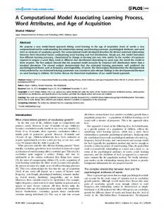
Figure 1. Overview of Fine-Tracker: the output of the prelexical level, consisting of a set of MLPs, is the input to the word ‘Search’ module at the lexical level. Figure 1 shows an overview of Fine-Tracker’s two levels. The prelexical level consists of a set of artificial neural networks, multi layer perceptrons (MLPs), which convert the continuous acoustic signal into feature vectors with a time resolution of 5 ms. At the lexical level, the feature vectors are used as input to the word search module, which is responsible for finding the word (sequence) that corresponds to the best path through the search space spanned by the prelexical feature vectors and the lexical representations. The output of Fine-Tracker is an Nbest list of most likely lexical paths with word scores for each word on each path.

2.1. The prelexical level The exact form of the prelexical representations is still a topic of research. In the absence of a clear answer, Fine-Tracker uses ‘articulatory features’ (AFs) as prelexical representations. This allows Fine-Tracker to ‘track’ phonetic detail in the speech signal and to model this subtle phonetic information. AFs describe acoustic correlates of articulatory properties of speech sounds (e.g. voice, nasality, roundedness, etc.) and can be used to represent the acoustic signal in a compact manner. Table 1 shows an overview of the AFs used by Fine-Tracker. Note that fr(ont)-back, round, height and dur(ation)diph(thong) only apply to vowels. Table 1. Specification of the AFs, their AF types, and the number of hidden nodes in the MLPs. AF AF type #hidden nodes manner plosive, fricative, nasal, glide, 300 liquid, vowel, si(lence) place bilabial, labiodental, alveolar, 200 (pre)palatal, velar, glottal, nil, sil voice +voice, -voice 100 fr-back front, central, back, nil 200 round +round, -round, nil 200 height high, mid, low, nil 250 dur-diph long, short, diphthong, nil 200

For each of the seven AFs, one MLP was trained for all its AF types using the NICO Toolkit [6], an artificial neural network toolkit designed for speech applications. For training, we used 3,410 randomly selected utterances from the manually transcribed read speech part of the Spoken Dutch Corpus (CGN; [7]). Each MLP consisted of three layers: an input, hidden, and output layer. The architecture of the MLPs was the same for all AFs, with the exception of the number of hidden nodes and number of output nodes. The hidden layers had hyperbolic tan transfer functions and a different number of nodes depending upon the AF. The optimal number of hidden units was determined through tuning experiments and is listed in the third column of Table 1. The output layer was configured to estimate the posterior probability of the AF type given the input. The number of output nodes is identical to the number of AF types (see Table 1). Speech files that were the input to the MLPs were parameterised with 12 Mel frequency cepstral coefficients (MFCC) and log energy, and augmented with first and second temporal derivatives resulting in a 39dimensional acoustic feature vector. The features were computed on 25 ms analysis windows with 5 ms frame-shift. The output of the prelexical level serves as the input of the lexical level of Fine-Tracker: for each input frame, each MLP creates a ‘soft’ decision, i.e., a continuous value between 0 and 1, for each of its AF types. This numeric value can be regarded as a measure of activation of this AF type (over time). Per input frame, the ‘soft’ decisions for each of the AF types are combined into a feature vector (see Figure 1), whose length is equal to the total number of AF types, resulting in a sequence of AF feature vectors with a time-spacing of 5 ms.

2.2. The lexical level The lexical representations of the words are based on the prelexical representations, so each word in the lexicon is represented in terms of AF feature vectors. Lexical feature vectors have the same dimension as the prelexical feature vectors (33), and each AF type in the lexical feature vectors takes a value between 0 and 1. Figure 1 shows an example of the lexical feature representations of the words ‘ham’ and ‘hamster’ in the lexicon of Fine-Tracker. Note that the phoneme labels at the start of each line representing a lexical feature vector are not used during the word search. It is possible to assign an ‘unspecified’ value to an AF type (this is indicated with an asterisk in the lexical representations in Figure 1): during the word search this AF type is ignored, meaning that the distance between this AF type in the lexical representation and its twin in the prelexical feature vector is not incorporated in the equation to determine the “goodness of fit” or distance (see below) between the two vectors. As the lexical AF types can in principle take any value between 0 and 1, speech phenomena such as coarticulation, assimilation, and nasalization of vowels can be encoded in a gradual continuous way (instead of a binary decision). The lexicon is internally represented as a tree of feature vectors. When a node in the lexical tree is accessed, all words in the corresponding word-initial cohort are equally activated. Continuous word recognition is implemented through a loop over the lexical tree. Essential in Fine-Tracker is the fact that the number of feature vectors can be set in the lexicon for each lexical item separately, which can be used to accommodate for the durational differences between words. Figure 1 shows an example: each of the phonemes of ‘ham’ is represented using two identical feature vectors, while there is only one feature vector per phoneme for the first syllable of ‘hamster’. Currently, the number of lexical feature vectors is set by hand.

The word search module of Fine-Tracker is able to deal with the resulting subtle differences in lexical representations. The ‘activation and competition process’ is implemented in the word search module (see Figure 1). It compares the prelexical feature vectors with the candidate words in the lexicon in order to find the most likely (sequence of) words by determining the word sequence with the smallest distance through the search space spanned by the prelexical and the lexical feature vectors. The segmentation of the acoustic signal into words is the result of the word search module; there is no explicit segmentation algorithm. Each word hypothesised by the search module is assigned a score that corresponds to the degree of match of the word to the current input, i.e., the already processed prelexical feature vectors. The word score is the score from the beginning of the word up to that point and is defined as follows: word _ score =

SV + α DM

(1)

prelex _ feature _ vectors

where, the step value (SV) is either the step-in-input or the step-in-input-and-lexicon parameter: • Step-in-input (SI): a value associated with making a ‘step’ in the input but not in the lexicon. • Step-in-input-and-lexicon (SIL): a value associated with making a ‘step’ in both the input and the lexicon. • Distance measure (DM): currently, the averaged squared distance between the prelexical and lexical feature vector. The relative weight of the acoustic distance measure DM is determined by a distance weight parameter . Also, the path on which each word lies is assigned a score. The path that has the lowest score has the best fit with the input. The path score then is the (sum of the) word score(s) accumulated with: • Word entrance penalty (WEP): cost to start a new word, i.e., the algorithm goes through the start of the lexical tree. • Word-not-finished penalty (WNF): at the end of the input, i.e., when all prelexical feature vectors have been processed, all activated cohorts that do not correspond to words get a penalty. This is to penalise incomplete word hypotheses alive at the end of the acoustic input. • History: the cost of the cheapest path from the beginning of the utterance up to the current search space node. The word search algorithm is time-synchronous and breadth-first: all search space nodes at a given time are expanded before the child search space nodes are created. The search algorithm allows a many-to-one mapping, so as to be able to map multiple 5 ms feature vectors onto a single lexical feature vector. During the search, it is possible to skip lexical feature vectors to accommodate for reductions and deletions. To restrict the search space, like in automatic speech recognition systems (see [8] for an overview), only the most likely candidate words and paths are considered. To that end, there is a maximum number of search space nodes kept in memory during the word search. There are no duplicate paths; only the cheapest path of identical word sequences is kept. At any moment in time, Fine-Tracker can produce a ranked N-best list of alternative parses, each with its associated path score. Each path (or parse) contains words, word-initial cohorts (can only occur as last element), silences, and any combination of these, and the word score for each of these items. In order to relate the output to behavioural data, an important assumption of any model is a measure of how easy each word will be for subjects to respond to in a listening experiment. This measure is usually referred to as ‘(word) activation’. [9] presents a way to directly compute word activations from the word scores as output by Fine-Tracker.

Since word activations can be directly computed from the word scores, we used the raw word scores in the subsequent simulations, as this would give the exact same results as having used the word activations.

3. Simulations 3.1. Simulation 1: Lexical embedding In an eye-tracking study, [2] found that listeners use durational information to distinguish between the embedded word and its matrix word. In this simulation, we investigate whether durational cues help Fine-Tracker to distinguish embedded words from their matrix words, using the original acoustic stimuli from [2]. The stimuli consist of manipulated Dutch sentences, each containing a ‘target word’. The target word is a polysyllabic word of which the first syllable also constitutes a monosyllabic word (e.g., ‘hamster’ contains the ‘ham’). In constructing the target words, the first syllable was either cross-spliced from a monosyllabic word (e.g., ‘ham’; MONO condition) or from the first syllable from another recording of that target word (‘hamster’; CARRIER condition). In total, 28 target words were used. In their study, [2] found that there were significantly more fixations to pictures representing monosyllabic words if the first syllable of the target word had been replaced by a recording of the monosyllabic word than when it came from a different recording of the first syllable of that target word. Eye-tracking studies provide a sensitive measure of the time course of lexical activation in continuous speech [10]. If we then consider the amount of eye fixations of the participants in [2] as a degree of the word activation during word recognition, the output of Fine-Tracker can be compared with the behavioural data. We expect the embedded word’s activation in the MONO condition to be higher than the activation of the embedded word in the CARRIER condition. In Fine-Tracker, durational differences between words are coded in the lexicon. In the ‘no duration’ condition, the lexical feature representation of the embedded word and the first syllable of the matrix word are identical: each phoneme in the lexical representation is represented by one feature vector. In the ‘duration’ condition, the lexical representation of the monosyllabic word and the first syllable of the matrix word are different. The syllables were on average 265 ms in the MONO and 245 ms in the CARRIER condition [2]. This durational difference of 20 ms is equal to four prelexical feature vectors. To accommodate for this durational difference, each phoneme in the lexical representation of the monosyllabic word is represented by two identical feature vectors, while each phoneme in the first syllable of the matrix word is represented by one feature vector. The lexical representations are obtained by substituting all phonemes of a word’s phonemic representation with its AF vectors. The lexicon consists of 27,740 entries. To guide Fine-Tracker’s word search, we applied priors to the 61 words that occurred in the stimuli, thus limiting the search algorithm to these 61 words. For the simulations, the speech files are cut manually such that the cut-out stimulus consists of the target word. The stimuli are parameterised with 12 MFCC coefficients and log energy and augmented with first and second temporal derivatives resulting in a 39-dimensional feature vector. The features were computed on 25 ms windows shifted by 5 ms per frame. Fine-Tracker’s parameters were optimised on the MONO set, and subsequently tested on the CARRIER set to ensure maximum performance on both sets. These parameter settings were used in all simulations reported in this paper.

3.1.1. Results and discussion

In all conditions, all 28 target and 28 embedded words were found in the 50-best list output by Fine-Tracker. In order to investigate the strength of Fine-Tracker’s modelling ability and the effect of durational information, we compared the word activations over time of the embedded words in the MONO and the CARRIER conditions. In the ‘no duration’ condition, for 10 out of the 28 stimuli, the embedded word in the MONO condition had the highest word activation. This number increased substantially when using a lexicon that takes durational information into account: for 18 of the 28 stimuli, the embedded word in the MONO condition had the highest word activation. This improvement, however, was shown not to be significant (F(1,27)=3.531, p=0.071, effect size is 0.116) according to an ANOVA with two within subject factors with two levels each, i.e., condition (MONO and CARRIER) and lexicon (with and without duration). The input of the ANOVA consisted of the average word scores. Despite the difference in simulation performance not being significant, the duration lexicon is better set-up than the nonduration lexicon. In the latter, the lexical representations of the embedded words and the first syllable of the matrix words are identical. Consequently, Fine-Tracker is unable to distinguish between the embedded words and the first syllable of the matrix words as they are in the same word-initial cohort. In the duration lexicon, however, the durational differences between the embedded and matrix words are coded in the lexicon and the embedded and matrix words are necessarily in different word-initial cohorts. These differences in lexical representations result in different competition effects for the two duration conditions. We expect the best modelling results for Fine-Tracker for those stimuli where the durational difference between the monosyllabic word (MONO condition) and the first syllable in the matrix word (CARRIER condition) is greatest, as the durational information is greatest for those stimuli. This assumption was tested by statistically comparing the word score differences (as calculated for the ANOVA) between MONO and CARRIER for the duration lexicon with the durational differences between the monosyllabic word and the first syllable of the matrix word. A 1-tailed (bivariate) Pearson correlation, indeed, showed a significant correlation (p=0.024) between the per stimulus difference in syllable duration between the MONO and CARRIER conditions and the stimuli where Fine-Tracker had the best modelling results. Thus, like for listeners, durational information helps Fine-Tracker to distinguish the embedded words from their matrix words.

3.2. Simulation 2: Segment durations We further investigate Fine-Tracker’s ability to detect and use durational information during word recognition, this time with respect to differences in durations of a single segment. We use the acoustic stimuli from the eye-tracking study presented in [3]. They presented listeners with Dutch ambiguous sentences. For instance, two subsequent words could either be interpreted as ‘eens pot’ (once jar) or ‘een spot’ (a spotlight). The sentences were constructed such that the final [s] of ‘eens’ and the target word (in this example) ‘pot’ was constructed either through identity-splicing (the IDENT condition), where the [s] of ‘eens’ and the target word were spliced from another recording of that same target-bearing sentence, or through cross-splicing (the CROSS condition), where the ‘eens’ target word sequence was spliced from a phonemically identical sentence but where the [s] of ‘eens’ was produced as the first segment of an [s]-plosive cluster, in our example ‘spot’. The stimuli consisted of 20 Dutch sentences each containing one

stop-initial ‘target’ word, the stop being either a [t] or a [p], preceded by the word ‘eens’ (once). [3] showed that the crucial difference between the two types of sentences was the duration of the [s], and that participants used the duration of [s] as a cue for placing the word boundary. In this simulation, we test Fine-Tracker on its ability to detect segmental durational cues that distinguish word final from word onset [s] realisations, and use these cues to place the word boundaries. Fine-Tracker’s task is to reproduce the findings that listeners are slower to fixate the picture of the target word when the duration of the [s] in the ambiguous sequence is longer, and that listeners made fewer fixations to the target picture in the CROSS condition than in the IDENT condition. Considering the amount of fixations of the participants as a degree of the word activation, we expect the activation of the target word in the CROSS condition generally to be lower than in the IDENT condition. We follow the set-up of the simulations as used in the previous simulation. However, since the duration lexicon is inherently better set-up than the non-duration lexicon, we only use a lexicon that contains durational information. Like in the previous simulations, each phoneme in the canonical lexical representation of the words was represented by a single feature vector, apart from the word-initial [s]. Praat (www.praat.org) measurements showed that the mean [s] duration in the IDENT condition was 88 ms and in the CROSS condition 105 ms. Taking this durational difference into account, word-initial [s] was represented by three feature vectors in the lexicon, while word-final [s] was represented by one feature vector. The stimuli were cut manually such that the cut-out stimulus consisted of the ‘eens’ followed by the target word sequence. Subsequently, the stimuli are parameterised with 12 MFCC coefficients and log energy and augmented with first and second temporal derivatives resulting in a 39-dimensional feature vector. The features were computed on 25 ms windows shifted by 5 ms per frame. Finally, like in the previous set of simulations, we applied priors to the 42 words in our stimuli.

3.2.1. Results and discussion

For both conditions, all 20 target words were found in the 50best list. We then compared the word activation over time of the target words in the IDENT and the CROSS condition. For 14 out of 20 stimuli, the target word had the highest word activation in the IDENT condition. For an additional two stimuli, the word activation of the target word was initially lower in the CROSS condition than in the IDENT condition, even though eventually the word activation of the target word in the CROSS condition grew higher than in the IDENT condition. The word activation of the target word thus grew slower in the CROSS condition than in the IDENT condition, as was found for the listeners in [3]. Like in the previous simulation, the difference in average word score between the IDENT and the CROSS conditions was compared with the difference in duration of the [s] in the IDENT and the CROSS condition. A 1-tailed (bivariate) Pearson correlation, showed a significant correlation (p=0.034) between the per stimulus difference in [s] duration and the stimuli where Fine-Tracker had the best modelling results. Fine-Tracker is thus also able to capture durational cues at the segment level and use it to its benefit during word recognition.

4. General discussion and conclusion Two simulations were carried out using the acoustic material from the original behavioural studies. The results showed that durational cues, like for humans, help Fine-Tracker to disambiguate temporary ambiguous phoneme sequences.

Durational cues allowed Fine-Tracker to distinguish embedded words from their matrix words (first set of simulations), and to distinguish word final realisations of [s] from word initial realisations (second simulation). Following the accumulated evidence that durational cues seem to play a major role in lexical interpretation, FineTracker only used durational information to differentiate between words. However, it is possible that listeners, in addition to duration, also use other cues, such as formant frequency information, assimilation cues, or relative durations within the span of the syllable to differentiate between possible interpretations of an ambiguous speech signal. More research is therefore needed to investigate the exact nature of the acoustic cues, besides duration, that play a role in the disambiguation process during spoken-word recognition. Incorporation of these possible other cues into Fine-Tracker might result in an improvement in modelling power. To conclude, Fine-Tracker is the first computational model of spoken-word recognition that, like humans, takes benefit from durational cues during word recognition. It is able to use durational cues in the acoustic signal to resolve temporarily ambiguous speech signals. As durational information is the only cue available to Fine-Tracker to make lexical and segmental distinctions between ambiguous phoneme sequences, it provides support for the theory that durational information plays a role in spoken-word recognition.

5. Acknowledgements This research was supported by a Veni-grant from NWO. The author would like to thank A.P. Salverda, J. McQueen, and K. Shatzman for kindly providing the acoustic data, and L. Boves for useful comments on an earlier version of this paper. The Fine-Tracker software is implemented in JAVA and is distributed via http://www.finetracker.org.

6. References [1]

Andruski, J.E., Blumstein, S.E., Burton, M., “The effect of subphonetic differences on lexical access”, Cognition, 52:163187, 1994. [2] Salverda, A.P., Dahan, D., McQueen, J.M., “The role of prosodic boundaries in the resolution of lexical embedding in speech comprehension”, Cognition 90, 51-89, 2003. [3] Shatzman, K.B., McQueen, J.M.. “Segment duration as a cue to word boundaries in spoken-word recognition”, Perception & Psychophysics 68, 1-16, 2006. [4] Scharenborg, O., “Modelling fine-phonetic detail in a computational model of word recognition”, Proc. Interspeech, Brisbane, Australia, pp. 1473-1476, 2008. [5] Norris, D., “Shortlist: A connectionist model of continuous speech recognition”, Cognition 52, 189-234, 1994. [6] Ström, N., “Phoneme probability estimation with dynamic sparsely connected artificial neural networks”, The Free Speech Journal, 5, 1997. [7] Oostdijk, N., Goedertier, W., Van Eynde, F., Boves, L., Martens, J.-P., Moortgat, M., Baayen, H., “Experiences from the Spoken Dutch Corpus project”, Proc. LREC, Las Palmas, Gran Canaria, pp. 340-347, 2002. [8] Ney, H., Aubert, X., “Dynamic programming search: From digit strings to large vocabulary word graphs”, In Lee, Soong, Paliwal (Eds.), Automatic speech and speaker recognition (pp. 385– 413). Boston: Kluwer Academic, 1996. [9] Scharenborg, O., Norris, D., ten Bosch, L., McQueen, J.M., “How should a speech recognizer work?” Cognitive Science 29 (6), 867-918, 2005. [10] Tanenhaus, M.K., Magnuson, J.S., Dahan, D., Chambers, C., “Eye movements and lexical access in spoken-language comprehension: Evaluating a linking hypothesis between fixations and linguistic processing”, Journal of Psycholinguistic Research 29(6), 557-580, 2000.