This multi-strategy system, called HAMLET-EVOCK, combines a learning algorithm ... Some of them learn global heuristics such as macro-operators [10,19,.
Using genetic programming to learn and improve control knowledge Ricardo Aler ∗ , Daniel Borrajo, Pedro Isasi Escuela Politécnica Superior, Universidad 30, 28911 Leganés, Madrid, Spain Received 28 March 2000; received in revised form 11 April 2001
Abstract The purpose of this article is to present a multi-strategy approach to learn heuristics for planning. This multi-strategy system, called H AMLET -E VO CK, combines a learning algorithm specialized in planning (H AMLET ) and a genetic programming (GP) based system (E VO CK: Evolution of Control Knowledge). Both systems are able to learn heuristics for planning on their own, but both of them have weaknesses. Based on previous experience and some experiments performed in this article, it is hypothesized that H AMLET handicaps are due to its example-driven operators and not having a way to evaluate the usefulness of its control knowledge. It is also hypothesized that even if H AMLET control knowledge is sometimes incorrect, it might be easily correctable. For this purpose, a GPbased stage is added, because of its complementary biases: GP genetic operators are not exampledriven and it can use a fitness function to evaluate control knowledge. H AMLET and E VO CK are combined by seeding E VO CK initial population with H AMLET control knowledge. It is also useful for E VO CK to start from a knowledge-rich population instead of a random one. By adding the GP stage to H AMLET , the number of solved problems increases from 58% to 85% in the blocks world and from 50% to 87% in the logistics domain (0% to 38% and 0% to 42% for the hardest instances of problems considered). 2002 Elsevier Science B.V. All rights reserved. Keywords: Speedup learning; Genetic programming; Multi-strategy learning; Planning
1. Introduction Many interesting problems in Artificial Intelligence can be formulated in terms of search in a state space: optimization, planning, machine learning, etc. In order to explore * Corresponding author
E-mail address: aler@inf uc3m es (R Aler)
1
efficiently such (usually huge) state-spaces, different Machine Learning (ML) techniques have been devised. Some of them learn global heuristics such as macro-operators [10,19, 32], “chunks” [37], or cases [13,14,41]. Other techniques learn local search heuristics (or control knowledge) [8,26]. All machine learning algorithms have biases that determine how they generalize to unseen instances [38]. Sometimes it is desirable that they possess other learning biases. However, it might be difficult to add those biases if the ML algorithm is very specialized. In this paper we intend to use Evolutionary Computation (EC) techniques to flexibly add those biases to an existing ML technique. EC includes methods such as Genetic Algorithms [12], Classifier Systems [12,34] and Genetic Programming (GP) [20]. EC algorithms explore concept spaces using different biases to other ML methods, as we will discuss throughout the paper. Also, some of the EC techniques learning biases can be declaratively stated in an evaluation function—the fitness function. In this article we combine an ML and an EC technique to learn symbolic heuristics in a complex search domain: planning. In particular, we propose a two-stage loosely coupled multi-strategy system (H AMLET-E VO CK), that learns control knowledge for P RODIGY 4.0, a means-ends bidirectional planner [39]. The first stage—H AMLET—is an incremental deductive-inductive multi-strategy system itself, built by Borrajo and Veloso [5]. The second stage (E VO CK: Evolution of Control Knowledge) is a GP based system whose purpose is to add corrective biases to H AMLET [1]. H AMLET-E VO CK is loosely coupled in the sense that the output of the first stage is just fed into the second stage, by seeding the GP initial population, instead of starting from a random one. The goal of the H AMLET deductive subcomponent is to obtain approximately correct control knowledge by means of Explanation Based Learning techniques (EBL) [26], while the aim of the inductive subcomponent is to incrementally refine it. However, we have found out that H AMLET does not always generate more accurate control knowledge by observing more and more examples. We suspect that this is due to its example-driven operators (like AQs [24]). This means that the only way H AMLET can refine current control knowledge is by being presented the proper set of examples. Unfortunately, if the examplespace is large, it could take H AMLET very long to generate correct control knowledge. Additionally, as H AMLET EBL subcomponent learns from search trees, preferably fully expanded, it has to be trained with simple planning problems. It might be the case that the examples needed to refine the control knowledge do not even exist in that subspace of planning problems. Our most important guiding hypothesis for this paper is that even though H AMLET can produce incorrect control knowledge, it is only partially incorrect. This means that it could be used with profit by other ML technique which moves through the concept space using complementary biases (this is our second hypothesis). For this purpose, we use GP, whose learning operators (mutation and crossover) do not require examples to modify its candidate hypotheses and therefore it is not limited by significant examples being rare. Our GP based control knowledge learner, E VO CK, is able to use additional non-exampledriven operators besides mutation and crossover. As usual, such operators are blind, and therefore E VO CK can also benefit from being combined with an example-driven system. Also, we use E VO CK fitness function to measure some properties of the control knowledge that cannot be easily assessed by H AMLET. At its best, H AMLET tries to obtain 2
control rules which are as general and correct as possible, but it is not concerned with rules being useful or simple. With respect to usefulness, an incremental system like H AMLET gives equal weight to all training problems whereas in some cases it might be desirable to ignore some of them if that helps to solve many other problems. This is easily achieved by E VO CK using a fitness function that counts the number of problems solved in a given time limit. With respect to simplicity, H AMLET tends to generate a lot of control rules. But having many control rules slows P RODIGY 4.0 down. Again, it is very easy to include a term in the fitness function so that the complexity of the control rules is reduced. One could think that simply doing an utility analysis (similar to P RODIGY 4.0-EBL [26]) would be enough for solving these problems. As we show with some experiments, in which rules are removed from the set of control rules according to the fitness function, this does not solve completely the problem. This paper is structured as follows. Section 2 comments on learning heuristics for planning. Section 3 describes in detail H AMLET-E VO CK, our multi-strategy architecture. Empirical results showing that the multi-strategy approach improves on the mono-strategy one will be shown and analyzed in Section 4. This will be followed by Related Work in Section 5, Conclusions in Section 6 and Future Lines of Work in Section 7.
2. The learning task Classical planning methods always involve search. Applying control knowledge at decision points in a search algorithm can yield far better performance than brute-force search. However, providing the “right” control knowledge is usually very hard for humans for they have to understand the way in which the planner works. The purpose of this article is to automatically learn and improve control knowledge for a classical planning system: P RODIGY 4.0. P RODIGY 4.0 searches a state-space bidirectionally, from an initial situation S towards the goals G, and vice versa [39]. P RODIGY 4.0 uses an augmented STRIPS representation. We could have chosen any other planner for this study, given that all planners (even the most sophisticated ones such as Blackbox [18] or Graphplan [4]) involve some kind of search. We decided to use P RODIGY 4.0 for its simplicity for introspection and for having a well integrated control knowledge module. P RODIGY 4.0 follows a four step decision cycle, as shown in Table 1. (1) First, the system must decide whether to apply the applicable planning operators to the current situation S (forward mode), or to work on a goal in G (backward mode). If in forward mode, the first currently applicable operator is applied.1 If in backward mode, (2) an unachieved goal g ∈ G must be selected. Then, (3) an operator O able to fulfill g must be chosen. And finally, (4) its unbound variables must be bound. Each one of these four decision points are backtracking points. P RODIGY 4.0 allows to define control rules to help the planner to take the right alternative at those points and avoid backtracking. Control rules can select, reject or prefer alternatives at decision points. Fig. 1 shows an example of a control rule for the blocks world domain. 1 In the latest versions of P RODIGY 4 0, this is also a decision point, that determines which ground operator will be applied We do not consider it in this article, though
3
Table 1 P RODIGY 4 0 four step decision cycle Procedure Prodigy-base (S, G) S, G are the current situation and goals, respectively g is a goal O is an unground operator Ob is a ground operator b is a binding • (1) Decide whether to work in forward or in backward mode: · If in forward mode, apply to S one of the ground operators whose preconditions are true in S · If in backward mode: (2) Select a goal g ∈ (G − S) (3) Select an operator O that can satisfy g (4) Select a binding b for grounding O G ← G ∪ preconds(Ob )
(control-rule select-operators-unstack (if (and (current-goal (holding )) (true-in-state (on )))) (then select operator unstack)) Fig 1 Example of a control rule for selecting the unstack operator in the blocks world If (holding ) is to be achieved, and it is currently true that block is on block , then the planner should select UNSTACK to achieve that goal
This control rule says that if P RODIGY 4.0 is working on trying to hold an object, ,2 (this is a goal in G) and this object is on top of another one, , in the current state S, then P RODIGY 4.0 should select the operator UNSTACK and reject the rest of operators that could achieve the same goal. In terms of search, this means that those successor nodes that are not related to the UNSTACK operator should be pruned.
3. H AMLET-E VO CK: A multi-strategy approach H AMLET-E VO CK is a multi-strategy system made of two different learning systems: H AMLET and E VO CK. H AMLET is an incremental example-driven method for learning control rules for planning, and E VO CK is the module that implements the GP paradigm adapted for searching in the space of sets of control rules. The first two subsections describe H AMLET, GP and the advantages of combining such different paradigms in terms of complementary biases. Section 3.3 describes how they are actually combined. Finally, Sections 3.4, 3.5, and 3.6 explain in detail E VO CK learning biases. 2 Variables are represented within < and >
4
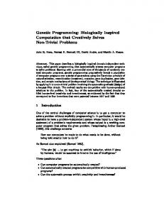
Fig 2 H AMLET high level architecture Inputs to H AMLET are: the domain description D, the set of training problems P , and other learning parameters L H AMLET outputs control knowledge C
3.1. H AMLET H AMLET is an incremental learning method based on EBL [25] (Explanation Based Learning) and inductive refinement [5]. Fig. 2 shows H AMLET modules and their connection to P RODIGY 4.0. The inputs to H AMLET are a task domain description (D), a set of training problems (P ), and other learning-related parameters (L).3 The output is a set of control rules (C). H AMLET has two main modules: the Bounded Explanation module, and the Refinement module. For each p ∈ P , H AMLET makes a first call to P RODIGY 4.0 with D, p, and the control knowledge C learned in previous cycles (initially C is empty). The Bounded Explanation module analyzes the resulting search tree ST . From the right decisions, this module generates a new set of rules that are added to the previous set C. Then, the Refinement module tries to generalize rules that have the same right hand side. H AMLET calls P RODIGY 4.0 again with the control rules learned so far C. After solving the same problem, P RODIGY 4.0 generates the search tree STC . From the wrong decisions made by the rules, the Bounded Explanation module generates negative examples that are stored for future use by the Refinement module. Also, since the generalized rules might cover previously found negative examples, the Refinement module specializes them to avoid that situation. We refer to [39] for further details about H AMLET. H AMLET has been tested in several domains: the standard blocks world and the logistics domain [5], some variations of them [3], and other domains such as a process planning domain, a work-flow domain, and a satellite control domain (results not published yet). H AMLET usually helped to improve the efficiency of the base-level problem solver as well as the quality of the solutions. However, H AMLET suffers from some weaknesses. 3 H AMLET is also able to use a plan quality metric In this article we use the standard quality metric (minimizing the number of operators in the plan) It is not included in Fig 2 to avoid cluttering it
5
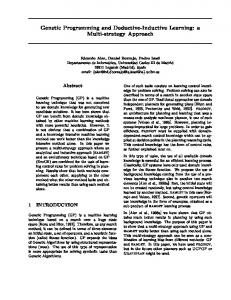
Fig 3 Learning curve for H AMLET in the blocks world and the logistics domain It also displays the evolution of the number of learned rules in both domains
In order to show them graphically, the following experiment was carried out. H AMLET was trained with 600 problems (with one or two goals) in two domains: the blocks world and the logistics domain. Every 50 problems, the rules obtained were tested with 416 and 346 testing problems (in the blocks world and the logistics domain, respectively). Testing problems are much harder (difficulty varies from 5 to 50 goals), to check generality. Fig. 3 displays the evolution of the proportion of testing problems solved and the number of rules learned in both domains. Fig. 3 shows that, although H AMLET is able to learn control rules that improve accuracy, some training problems can decrease it. Also, even after having seen 600 problems, the best control rules returned by H AMLET are able to solve only 54% of the testing problems in the blocks world, and 47% in the logistics domain, within a reasonable time limit.4 We believe that the main reason behind this behavior is due to H AMLET example-driven operators. In order to refine an incorrect control rule, H AMLET assumes that eventually it will find an appropriate set of positive and negative examples. Example-driven operators seem a good heuristic, but given that the potential problem space is huge, the likelihood of finding the appropriate set of problems might be very small in some cases, and learned rules might remain partially correct for a long time. Furthermore, because H AMLET requires preferably fully expanded search trees, learning is limited to simple problems. However, the examples needed to refine the control rules might not even exist in the subspace of simple problems. Additionally, H AMLET—as any other incremental system—has no global picture of the usefulness of the learned control knowledge. It considers all training problems equally, whereas in some cases it might be desirable to ignore some of them if 4 Here, we use the same time limit as in Section 4 1: 150 (1 + floor( #goals )) 16 10
6
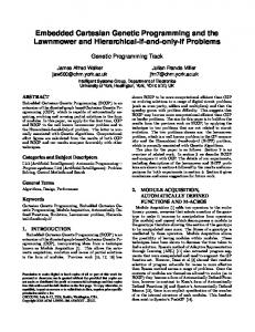
that helps to solve many other problems. The previous analysis should not be considered a complete diagnostic, but a guiding hypothesis for this article. Fig. 3 also displays the evolution of the number of learned rules. It shows that H AMLET has a strong tendency to increase the number of control rules (up to 16 rules in the blocks world and 91 in the logistics domain) even though this does not always improve the number of testing problems solved. The more rules there are, the longer it takes to evaluate them, so this should be avoided, if possible. Also, it can be observed that there is not a direct correlation of number of learned rules and performance decrease, as usually happens in utility analysis. We hypothesize that although H AMLET control knowledge is sometimes incorrect, it is only partially incorrect, and could be corrected and improved by means of other learning system with complementary biases. Based on this assumption, we have chosen to combine H AMLET with GP because it possesses the appropriate biases. It is not example-driven and not incremental; and it can evaluate the usefulness and compactness of hypotheses. GP is described in the next section. 3.2. Genetic programming GP is an Evolutionary Computation (EC) method that has been used for program induction and machine learning [20]. GP searches in the space of computer programs, trying to find a “good enough” computer program according to some metric. GP is a kind of Beam Search [36]. It maintains a set (or population) of many computer programs (or individuals), each one usually represented as a parse tree. GP search is guided by a heuristic (or fitness) function. It measures how well a computer program performs, according to a set of user defined fitness cases. Standard GP uses three search genetic operators: reproduction, mutation, and crossover. Reproduction copies an individual without changes. Mutation replaces a subtree of the individual by another randomly generated one. Crossover swaps two randomly chosen subtrees from two different individuals, as shown in Fig. 4. Table 2 depicts the algorithm followed by steady-state GP, which is the variety used in this work. One important aspect of the previous algorithm is the selection of individuals for reproduction and for replacement. The most common selection method chooses individuals with a probability proportional to their fitness. Another method—tournament selection— selects randomly a subset of individuals in the population and returns the best one (or the worst, in case of replacement).
Fig 4 The crossover operator swaps two subtrees randomly chosen
7
Table 2 Steady state GP algorithm Function steady-state GP (AO, → p AO , f ) AO contains the available genetic operators → p AO is a vector containing the probabilities of selecting each operator f is the fitness function P is the genetic population G is a genetic operator I1 , I2 , and I3 are individuals (1) Create P containing random individuals (2) Assign a fitness value to each individual in P using f (3) Repeat until some termination criterion is satisfied: p AO (a) Select G from AO according to → (b) Select I1 from P according to its fitness IF G is crossover, select also I2 Better individuals are more likely to be selected (c) Select I3 from P to be replaced Worse individuals are more likely to be selected (d) Apply G to I1 (and to I2 if the operator selected was crossover) and replace I3 with it
In contrast to H AMLET, GP follows a generate-and-test approach to modify hypotheses (mutation and crossover), instead of being example-driven. GP is not incremental either. Also, the fitness function can evaluate individuals for usefulness, compactness, etc. On the other hand, E VO CK learning operators do not contain as much knowledge about learning in the planning domain as those of H AMLET. Therefore, GP might also benefit from the combination. Next section explains how this is achieved. 3.3. H AMLET-E VO CK This section explains how H AMLET and E VO CK are combined in the multi-strategy system H AMLET-E VO CK. Fig. 5 displays its basic architecture. H AMLET, P RODIGY 4.0, and the problem generator are preexisting modules. Training H AMLET-E VO CK occurs in two stages. First, H AMLET learns a set of control rules from a training set randomly generated by the problem generator. Then, they are used to seed E VO CK initial population. E VO CK tries to evolve H AMLET set of control rules by using a second training set (also generated by the problem generator). P RODIGY 4.0 is used differently by the two learning systems. H AMLET sends the training problems to P RODIGY 4.0, which solves them, and sends back the search trees, from which H AMLET can learn, as explained in Section 3.1. E VO CK uses P RODIGY 4.0 to evaluate its individuals (each individual is a set of control rules). For that purpose, individuals are loaded into P RODIGY 4.0 and then [P RODIGY 4.0 + individual] is run on the training problems (or fitness cases). Performance data such as whether the problems were solved or not, or the time required to solve them, is returned to E VO CK. This is used to determine the worth (fitness) of the individual to guide selection. E VO CK can also learn starting from a random population, as in standard GP. When E VO CK finishes, it returns its best individual. The next three subsections describe E VO CK by explaining its learning biases according to Utgoff [38] (language, exploration, and evaluation biases). 8
Fig 5 Architecture of H AMLET-E VO CK First, H AMLET learns control rules from problems generated by the problem generator (L are H AMLET learning parameters) H AMLET rules are used to seed E VO CK initial population Then, E VO CK tries to improve them by using new training problems P RODIGY 4 0 is used by E VO CK to evaluate individuals
3.4. The language bias Any learning system is biased by the language that is used to represent candidate hypotheses and examples. In the case of GP, individuals represent the hypotheses and in our case, we decided that each individual represents a set of control rules. Each of the control rules has two parts, the left hand side (LHS) and the right hand side (RHS). The LHS contains a list of conditions that need to be true for the rule to be applied. The RHS specifies the decision to be made. Each condition calls a meta-predicate, which are functions that have access to P RODIGY 4.0 internal state. The meta-predicates used in this paper are: • true-in-state(fact): it tests if fact is true in the current planning situation S. • current-goal(goal): it checks if goal is the current goal the planner is working on. • target-goal(goal): it tests whether goal is one of the pending goals in G. • some-candidate-goals(goal1, goal2, . . . ): it is equivalent to: target-goal (goal1) ∨ target-goal (goal2) ∨ . . . . Usually, in GP there are no constraints on the structure to evolve: any combination of functions and terminals is valid. This is called operational closure [20]. However, in E VO CK case, P RODIGY 4.0 constrains the syntax of the control rules. Also, metapredicates must be supplied with the right type of arguments. And more importantly, it is a waste of search time to create expressions that are known not to be valid in the first place. Therefore E VO CK individuals are constrained to P RODIGY 4.0-valid ones (in the literature, such structures are called constrained structures [20] or strongly typed structures [27]). Actually, E VO CK individuals are constrained by the same sublanguage than H AMLET (select, apply, and sub-goal rules, and the same meta-predicates). In order to achieve this, only valid individuals must be created in the initial population. Also, applying a genetic operator to valid individuals must produce valid individuals. 9
Table 3 Domain independent grammar for generating syntactically correct sets of control rules LIST-ROOT-T is the axiom of the grammar → → → →
LIST-ROOT-T RULE-T AND-T METAPRED-T
LIST-OF-GOALS-T → ACTION-T →
(list RULE-T) | (list RULE-T RULE-T) | (rule AND-T ACTION-T) (and METAPRED-T) | (and METAPRED-T METAPRED-T) | (true-in-state GOAL-T) | (target-goal GOAL-T) | (current-goal GOAL-T) | (some-candidate-goals LIST-OF-GOALS-T) (list-goal GOAL-T) | (list-goal GOAL-T GOAL-T) | (select-goal GOAL-T) | (select-operator OP-T) | (select-bindings BINDINGS-T) | sub-goal | apply
Table 4 Domain dependent grammar for generating syntactically correct sets of control rules in the logistics domain E VO CK is able to automatically generate this grammar from the domain description OP-T
→
BINDINGS-T
→
GOAL-T
→
load-truck | load-airplane | unload-truck | unload-airplane | drive-truck | fly-airplane (load-truck-b OBJECT-T TRUCK-T LOCATION-T) | (load-airplane-b OBJECT-T AIRPLANE-T AIRPORT-T) | (unload-truck-b OBJECT-T TRUCK-T LOCATION-T) | (unload-airplane-b OBJECT-T AIRPLANE-T AIRPORT-T) | (drive-truck TRUCK-T LOCATION-T LOCATION-T) | (fly-airplane AIRPLANE-T AIRPORT-T AIRPORT-T) (at-truck TRUCK-T LOCATION-T) | (at-obj OBJECT-T LOCATION-T) | (inside-truck OBJECT-T TRUCK-T) | (inside-airplane OBJECT-T AIRPLANE-T)
The creation of valid individuals is achieved by using two special-purpose production grammars: domain independent (shown in Table 3) and domain dependent (shown in Table 4). This second grammar is generated on-the-fly by E VO CK for any domain described in P RODIGY 4.0 Description Language [6].5 The grammar shown in Table 4 is for the logistics domain, a well known planning domain described in [40]. In this domain, packages have to be delivered to several locations using trucks (inside a city) or airplanes (between cities). Terminal symbols in the grammars are displayed in lowercase and non-terminal generative symbols are shown in uppercase. This grammar has production rules that follow the structure A → (Fa A1 A2 . . .)|(Fb B1 B2 . . .)| . . . , where Fa is a terminal and Ai , Bi , . . . are either terminals or non-terminals. They generate lisp sentences such as (Fa A1 A2 . . .). A whole individual is generated by starting with the LIST-ROOT-T symbol, and randomly applying the production rules until an individual is completed. As it can be seen, each individual is a list of control rules. 5 Some non-terminal symbols, like OBJECT-T, do not appear in the grammar They only generate terminal symbols like , , , which are control rule variables This is also true for TRUCK-T, CARRIER-T, AIRPLANE-T, LOCATION-T, AIRPORT-T, and POST-OFFICE-T
10
Besides being able to generate valid individuals for the initial population, E VO CK genetic operators need to transform valid individuals into valid individuals. For mutation, the process is similar to creating a whole individual. First, the mutation point is randomly selected (as in standard mutation). Then, E VO CK determines which non-terminal symbol generated the element at the mutation point. This is achieved by checking the right hand side of the productions, and comparing them with the element at the mutation point. For instance, if the element at the mutation point was and, then its non-terminal generative symbol would be AND-T, as the third production of the grammar in Table 3 indicates. Finally, it replaces the subtree at the mutation point by a randomly grown one by applying the production rules from the non-terminal symbol (AND-T, in this case). This mechanism enforces that the new subtree is of the same type than the old one, which is enough in this case to assure correctness. Constrained crossover works likewise. First, a crossover point is selected randomly in the mother individual. Then, the non-terminal symbol that generated it is determined. Next, a crossover point that was generated with the same symbol is randomly selected in the father individual. Finally, both subtrees are swapped, as in standard crossover, to produce the offspring. 3.5. The exploration bias The exploration bias deals with the way in which the learning algorithm explores the search space. E VO CK uses the standard GP operators and some others specially tailored for this learning task. All of them use a grammar to always produce correct individuals, as explained in Section 3.4. Besides constrained mutation and crossover, E VO CK uses the following operators: • Adding Crossover: it takes a rule (RULE-T) or a goal (GOAL-T) from an individual and adds them to another individual at LIST-ROOT-T and LIST-OF-GOALST points, respectively. This operator adds subtrees to individuals, whereas standard crossover replaces them. • Growing mutation: it adds a randomly generated rule (RULE-T) or goal (GOAL-T) at points generated by LIST-ROOT-T and LIST-OF-GOALS-T, respectively. It is equivalent to adding crossover with a randomly generated individual. • Chopping off mutation: a randomly selected rule or goal is pruned from the individual. • Join: it selects one variable in the control rule (like ) and substitutes it by any other variable in the control rule that already exists. The rationale behind this operator is that sometimes there are conditions in a rule that are not related with other conditions by common variables. This is usually undesirable. For instance, in the blocks world, if there is a control rule to pick-up an object when some other conditions are true, our experience says that many of those other conditions should refer to as well. The join operator is a simple way of creating these references. E VO CK can also seed its initial population to focus the search, as explained in Section 3.3. 11
3.6. The evaluation bias The evaluation bias concerns the preference criteria used by GP for selecting an individual over another, which is coded as a fitness function. This fitness function must reflect the goal of the system, which is to generate an individual that solves as many problems as possible (limited by a timeout or node limit)6 and faster than P RODIGY 4.0. To achieve this goal, a hierarchical fitness function has been devised [1]. A hierarchical function contains several components to be maximized (or minimized). Instead of using a weighted addition of the components to compare different individuals, a hierarchical function compares them using the first component. If there are draws, it uses the second component, and so on. There are other alternatives for multi-criteria optimization such as Pareto (see for instance [21]). We selected hierarchical functions because it is a simpler approach that does not require a big population to store the whole Pareto front. The components of E VO CK hierarchical fitness function are as follows: (1) Performance in training problems: to maximize. It contains three sub-components, ordered as follows: (a) Number of problems solved by the individual expanding strictly fewer nodes than P RODIGY 4.0: to maximize. (b) Number of problems solved by the individual: to maximize. (c) Total number of nodes expanded by the individual: to minimize. This is used instead of time because measured time varies slightly even when the system is run in similar conditions. This would make the process non-deterministic and experiments unrepeatable. (2) Number of different variables: to minimize. It relates to the same bias as the join operator. It is desired to have meta-predicates in the LHS inter-related by common variables. (3) Generality/Compactness: to maximize. Generality and compactness is encouraged by minimizing the number of restrictions in the LHS of the control rules (i.e., the number of true-in-state and some-candidate-goals (SCG) meta-predicates) and by maximizing the number of arguments of SCG (SCG is equivalent to a disjunction of meta-predicates. Therefore, the more arguments, the more general a control rule is). Further compactness is achieved by minimizing the number of control rules and the size in nodes of the individual. Component (1)(a) deserves a longer explanation. Training problems are necessarily easy; otherwise the time limit for fitness evaluation would be too large. However, P RODIGY 4.0 is able to solve easy problems without heuristics. Therefore, a good strategy for individuals to score well in the “number of problems solved” component (1)(b) is to do nothing at all and let the planner do all the work. This is very easy to achieve, for instance, by means of control rules with conditions that never match. On the other hand, individuals that do modify the behavior of the planner are likely to be only partially 6 The node limit is 4N , where N is the number of nodes required by P RODIGY 4 0 to solve the problem without backtracking
12
correct, and to solve fewer problems than the planner without any heuristics. Therefore, individuals that do nothing will be selected and those that modify the behavior of the planner will not, even though many of the latter might be corrected in the long term. To change this undesirable behavior, we added a first component that forced individuals to do something positive: solving problems using strictly fewer nodes than P RODIGY 4.0 (component (1)(a)). Individuals that do nothing will score 0 in this component and will be selected against. However, there is a risk: there can be some individuals that obtain a good score in this component but that solve fewer problems (they score poorly in the second component). This might happen, but in the long term it is expected that, once the first component cannot be improved further, the second component will take the lead and begin to be improved itself.
4. Empirical results The aim of this section is to describe how H AMLET-E VO CK has been tested. We will first describe how the experiments were carried out. Then, we will show the results and comment on them. 4.1. Experimental setup First, 400 problems in two planning domains (blocks world and logistics domain) were randomly generated to train H AMLET and obtain the H AMLET seed. Then 192/188 new training problems from the blocks world and the logistics domains, respectively, were randomly generated and used by E VO CK to evolve H AMLET seed. The training sets contain planning problems with 1 and 2 goals and from 2 to 5 objects (blocks in the blocks world and packages in the logistics domain). As GP is stochastic, E VO CK was run 50 times using the same H AMLET seed, but with a different random seed for the random number generator (i.e., 50 GP-runs). Finally, the best set of control rules from each run was evaluated with 416/346 testing problems (blocks world/logistics domain) randomly generated by the same problem generator. Those problems are much more difficult than the ones used for learning, so that scalability of the rules can be checked. The time limit #goals for testing a problem is calculated with the formula ttest = 150 16 (1 + floor( 10 )) seconds, where #goals is the number of goals in the testing planning problem. Testing was carried out on a 400 MHz Pentium II with 256 MB RAM. This experimental sequence corresponds to the thick line of Fig. 6 and will be referred to as H AMLET-E VO CK. Obtaining good results from the multi-strategy system is not enough. It is necessary to know what would have happened if all the training problems would have been given to H AMLET, instead of dividing them between the two components of H AMLET-E VO CK. If H AMLET alone produces better results than H AMLET-E VO CK, then the multi-strategy system is obviously not solving H AMLET deficiencies. Therefore, after learning with the first training set, H AMLET was fed with the second one. From them, H AMLET produced a new set of control rules, which was subsequently tested. This second experimental sequence is represented by the thin line of Fig. 6 and it will be referred to as H AMLETH AMLET because it uses H AMLET in sequence. 13
Fig 6 Description of the three different experimental configurations: multi-strategy H AMLET-E VO CK vs monolithic H AMLET-H AMLET and stand-alone E VO CK
Although it is not the focus of this article, another experimental configuration was carried out to compare the effects of seeding E VO CK initial population (that is, H AMLETE VO CK) with E VO CK starting from a random population, as in standard GP. This third experimental setup (dashed line in Fig. 6) will be referred to as E VO CK, because E VO CK is used as a stand-alone learning system. In both E VO CK and H AMLET-E VO CK, two different configurations were tried, with population sizes of 2 and 300, respectively (the respective tournament set sizes were 2 and 5. No crossover was used in the 2-population). However, the greedy configuration (2-population) significantly outperformed the more exploratory one in both domains.7 Therefore, in this paper we only report the results for the greedy configuration, so as not to clutter the results section. Both E VO CK and H AMLET-E VO CK were run for a maximum of 100000 evaluations (an evaluation is a call to P RODIGY 4.0 to evaluate an individual with a single training problem). 4.2. Results In this section, results of the three experimental configurations will be discussed and compared. The GP runs for the stand-alone configuration E VO CK and the multistrategy configuration H AMLET-E VO CK are summarized in Fig. 7. This figure is a cumulative frequency graph, that shows the frequency (y-axis) with which an experimental configuration yields a set of control rules that is able to solve a given percentage of problems or more (x-axis). This can be interpreted as an estimation of the probability an experimental configuration will produce an individual that solves, at least, a given percentage of problems. Results for P RODIGY 4.0 and H AMLET seed are also provided for comparison purposes (the dashed and continuous vertical lines in Fig. 7). Given that 7 It might be possible that larger populations (i e , more exploratory configurations) would give better results if given many more evaluations However, results obtained with 2 populations were so good that we did not try more computationally expensive experiments
14
Fig 7 Frequency of GP runs (y-axis) that are able to solve a proportion x of problems (x-axis) or more Results for the blocks world are on the left and for the logistics domain on the right
these two systems are not stochastic, they are represented by vertical lines. The purpose of these results is to visualize the effects of seeding E VO CK initial population with H AMLET seed. We have used approximate randomization to determine whether the differences between E VO CK and H AMLET-E VO CK shown in Fig. 7 are statistically significant [7]. In particular, for each frequency of solved problems (x-axis of graphics in Fig. 7) we calculated the probability that the differences between the cumulative frequencies of E VO CK and H AMLET-E VO CK are due to chance, at the 5% level. Results are analyzed as follows: • In the blocks world, the cumulative probability is always greater for H AMLET-E VO CK than for E VO CK (and this is statistically significant). This means that, for instance, it will take H AMLET-E VO CK fewer runs to find an individual that solves 40% of the problems. Also, it is clear that H AMLET-E VO CK improves over the seed supplied by H AMLET, as 90% of the runs do better than H AMLET alone. • This happens in the logistics domain as well: 93% of the GP-runs improve over H AMLET seed. However, the analysis of the cumulative frequency diagram is not so clear-cut as in the blocks world case. In the range (0%, 62%), H AMLET-E VO CK is able to find good individuals more frequently than E VO CK (and this is statistically significant). However, there are no significant differences in the range (62%, 100%). In fact, the best individuals are found by E VO CK. This might be due to chance, or to the fact that the H AMLET seed in the logistics domain is very large (56 rules), whereas E VO CK best individual contains only 3 rules. Therefore, it might be very time consuming for H AMLET-E VO CK to correct the H AMLET seed. In fact, it only manages to obtain a 21 rule individual. In the blocks world, the H AMLET seed is only 12 rules long, not very far away from the 5 rule best individual created by stand-alone E VO CK. 15
It could be thought that a simpler integration of H AMLET and GP would perform equivalently. After all, H AMLET has a way of creating rules, but no way of evaluating which ones to keep. E VO CK has both: constrained genetic operators for the former and the fitness function for the latter. What would happen if E VO CK fitness function was used to remove non-useful H AMLET seed rules?. It is possible that H AMLET is after all a better control rule generator, if only its control rules were filtered somehow, like the utility analysis carried out in [26]. In order to test this simpler approach, we have tried another configuration of the multi-strategy system where E VO CK can either prune rules or add rules that were already present in the H AMLET seed (no other genetic operators are allowed).8 Addition of rules provides a sort of backtracking mechanism, to test whether a control rule that had already been removed has some good effects once other rules have been removed. The effects of H AMLET-E VO CK with the restricted set of genetic operators have been labeled ’H AMLET + pruning’ in Fig. 7. In both domains, the cumulative curve is almost vertical, which means that in most runs H AMLET-E VO CK got an equivalent individual. This restricted multi-strategy configuration is able to improve H AMLET seed. If only the best individuals are taken into account (which are not very different from the worst ones), the H AMLET seed is improved by 7% in the blocks world and by 12% in the logistics domain (see also Table 5). These results allow to draw three important conclusions: • The H AMLET seed contains quite good control rules and therefore, it makes sense to use them as seed for H AMLET-E VO CK. • The H AMLET seed contains incorrect control rules (once removed, performance increases). In fact, in the logistics domain, the main source of power is pruning. The best individual from H AMLET + pruning solves 62% of the testing problems, and after that value, differences between E VO CK and H AMLET-E VO CK do not differ significantly (see Fig. 7). • However, mere pruning does not get as good results as full-fledged H AMLET-E VO CK. The “creative” aspects of GP are required as well (mutation, crossover, etc.). In summary, H AMLET-E VO CK is able to improve significantly H AMLET seed and to find good individuals (although not always the best ones) more frequently than E VO CK alone. But it is interesting to know whether H AMLET alone scores better when given all the training examples (i.e., the H AMLET-H AMLET configuration). The learning curve in Section 3.1 (Fig. 3) already hints that this will not necessarily improve H AMLET control rules. Table 5 shows that when H AMLET tries to refine and improve a set of control rules previously learned by itself (H AMLET seed in Table 5), the percentage of test problems solved actually drops: in the blocks world it falls from 58 to 18%, in the logistics domain it gets from 50 to 47%. This is a confirmation of the oscillatory behavior displayed in Section 3.1 (Fig. 3). On the other hand, H AMLET-E VO CK improves the set of control rules given as seed for the initial population: 58–85% in the blocks world and 50–87% in the logistics domain. Therefore, it seems that the multi-strategy system does better than the 8 Actually, it was one of the reviewers who suggested this experiment
16
Table 5 Results for P RODIGY 4 0, H AMLET seed, H AMLET-H AMLET, E VO CK (random seed), H AMLET-E VO CK, and H AMLET + pruning in the blocks world and logistics domains Blocks world
P RODIGY 4 0 H AMLET seed H AMLET-H AMLET E VO CK H AMLET-E VO CK (best ind ) H AMLET+Pruning (best ind )
Logistics domain
% Problems solved
Number of rules
% Problems solved
Number of rules
26% 58% 18% 80% 85% 65%
12 13 3 5 5
43% 50% 47% 98% 87% 62%
56 64 3 21 16
Fig 8 Proportion of problems solved when varying the testing time limit from 0 to 100% Results for the blocks world are on the left and for the logistics domain on the right
mono-strategy one. It is also noticeable that H AMLET-E VO CK produces individuals with fewer control rules than the seeding individual (12 to 5 control rules in the blocks world and 56 to 21 in the logistics domain) hence returning more efficient individuals. On the other hand, H AMLET-H AMLET always increases the number of control rules: from 12 to 13 in the blocks world and from 56 to 64 in the logistics domain. Thus, H AMLET-E VO CK provides the sought compactness bias to H AMLET. Segre et al. [33] critique an arbitrary choice of a time limit for testing. Fig. 8 displays how the proportion of problems solved increases when the allocated testing time goes from 0 to 100% of the maximum testing time limit ttest . If we had observed that the H AMLET seed or H AMLET-H AMLET solved more and more problems as the allocated time increased, and this did not happen for H AMLET-E VO CK, it should have been concluded that H AMLET would eventually outperform the multi-strategy system. However, Fig. 8 shows that this is not the case. Therefore, the reason of H AMLET-H AMLET drop in performance is not that it generates clever but slow to evaluate rules, but that they are not very correct rules. In order to show that the set of control rules learned are general and useful for more complex problems, a breakdown of the results is displayed in Tables 6 and 7. Problem 17
Table 6 Breakdown of the number of testing problems solved in the blocks world by H AMLET and E VO CK according to the number of goals and objects # Goals-# Objects 50-50 (4%) 20-50 (11%) 20-20 (11%) 10-50 (11%) 10-20 (11%) 10-15 (11%) 05-50 (10%) 05-20 (10%) 05-15 (10%) 05-10 (10%)
P RODIGY 4 0
H AMLET seed
H AMLET-H AMLET
H AMLET-E VO CK
E VO CK
0% 8% 10% 21% 25% 40% 18% 20% 42% 65%
0% 33% 29% 60% 56% 48% 70% 90% 88% 88%
0% 4% 4% 19% 15% 15% 2% 18% 38% 60%
38% 77% 73% 94% 85% 85% 92% 98% 98% 95%
31% 71% 65% 83% 75% 77% 88% 92% 95% 95%
Table 7 Breakdown of the number of testing problems solved in logistics domain by H AMLET and E VO CK according to the number of goals and objects # Goals-# Objects 50-50 (14%) 20-50 (9%) 20-20 (8%) 10-50 (4%) 10-20 (4%) 10-15 (4%) 10-10 (4%) 05-50 (3%) 05-20 (3%) 05-15 (3%) 05-10 (3%) 05-05 (3%) 02-50 (3%)
P RODIGY 4 0
H AMLET seed
H AMLET-H AMLET
0% 3% 7% 13% 20% 20% 7% 42% 58% 42% 25% 33% 90%
0% 0% 7% 0% 53% 67% 67% 0% 75% 42% 58% 83% 40%
0% 0% 0% 0% 33% 40% 40% 0% 67% 58% 67% 92% 40%
H AMLET-E VO CK 42% 87% 90% 80% 80% 87% 80% 83% 83% 67% 67% 100% 90%
E VO CK 77% 97% 100% 100% 100% 100% 100% 100% 100% 100% 100% 100% 100%
complexity is measured by the number of goals and objects in the planning problem. This is shown in the first column of Tables 6 and 7 (the quantity in parentheses represents the percentage of problems of that difficulty level there are in the testing set). Usually, the more goals and objects a problem has, the more difficult it is for the planner to solve it. The last assertion can be easily checked in Table 6, where results for P RODIGY 4.0 are supplied. For instance, P RODIGY 4.0 solves none of the 50-50 problems. H AMLET-E VO CK improves drastically with respect to the initial seed (H AMLET seed) by solving very hard problems (50 goals and 50 objects). The percentage of testing problems solved for P RODIGY 4.0 working alone and H AMLET-H AMLET results are also shown.9 9 In the logistics domain, results for the 2-20, 2-15, 2-10, 2-5, 2-2, 1-50, 1-20, 1-15, 1-10, 1-5, and 1-2 types are not shown because they are not very interesting They comprise about 33% of the testing problems E VO CK solves all of them and the other configurations solve most of them (percentages are always greater than 80%, and very often greater than 90%)
18
4.3. Learning curves In this section, we study experimentally how the performance of E VO CK and H AMLET-E VO CK changes when three important parameters are modified: the number of evaluations, the number of training examples, and the quality of the H AMLET seed. Due to GP being rather time expensive, these learning curves contain only three points (three cumulative frequency curves, actually) corresponding to three different parameter values. One of the three points represents the cumulative curve obtained from the default parameters that was already discussed in Fig. 7 of Section 4.2. The other two have been generated from 30 GP-runs each. This is true for all the graphs of this section. It is not easy to quantify whether one cumulative frequency curve is “better” than another. Here, we have decided to carry out an approximate randomization test like in Section 4.2. One curve is considered better than another if it has a significantly (0.05 level) higher probability of obtaining an individual that solves at least x% of the testing problems. x is the percentage of problems solved by H AMLET + pruning (this has been discussed previously in Table 5). x = 0.65 for the blocks world and x = 0.62 for the logistics domain. We have considered this a reasonably non-arbitrary way of focusing on the interesting part of the distributions (their upper tail). Figs. 9(a) and (b) show how the cumulative frequency graphs for E VO CK and H AMLET-E VO CK change when the number of evaluations increases from 33333 to 100000. Differences for E VO CK are not significant, which means that E VO CK had already converged at 33333 evaluations, and that no significant over-fitting occurs by allowing more evaluations. In the case of H AMLET-E VO CK, there are significant differences for the (66666, 33333) curves. Probably, H AMLET-E VO CK needs enough evaluations to correct the often complex H AMLET seed. Fig. 10 displays the same information for the logistics domain. In this case, E VO CK benefits from increasing the number of evaluations ((66666, 33333) are significantly different), although it seems to be converging at 100000 evaluations (no significant differences for the (100000, 66666) curves), as shown in Fig. 10(a). H AMLET-E VO CK also improves as evaluations increase, as shown in Fig. 10(b)
(a)
(b)
Fig 9 Cumulative frequency graphs of E VO CK (a) and H AMLET-E VO CK (b) for 33333, 66666, and 100000 evaluations, respectively (blocks world domain)
19
(a)
(b)
Fig 10 Cumulative frequency graphs of E VO CK (a) and H AMLET-E VO CK (b) for 33333, 66666, and 100000 evaluations, respectively (logistics domain)
(a)
(b)
Fig 11 Cumulative frequency graphs of E VO CK (a) and H AMLET-E VO CK (b) for 64, 128, and 192 examples, respectively (blocks world domain)
(significant differences for (66666, 33333)). The H AMLET seed in the logistics domain is even larger than in the blocks world, so this result makes sense. Figs. 11 and 12 display the cumulative frequency graphs when the number of training problems changes from 1/3 of the original training data, to 2/3, and 3/3, in the blocks world and the logistics domain, respectively. The number of evaluations has been reduced proportionally to keep evaluations per problem constant. Otherwise, decreasing the number of training problems to be processed for each individual would increase the number of GP generations and therefore, the number of applications of the genetic operators. In that case, it would be uncertain whether performance is different because fewer training problems were used, or because genetic operators were applied more times. Fig. 11(a) shows that E VO CK gives about the same result for 1/3, 2/3, and 3/3 of the examples. Indeed, approximate randomization shows that these differences are not significant. This means that E VO CK had already converged with only 1/3 of the training examples. This is the case also for H AMLET-E VO CK (see Fig. 11(b)). In the logistics domain, E VO CK 20
(a)
(b)
Fig 12 Cumulative frequency graphs of E VO CK (a) and H AMLET-E VO CK (b) for 62, 124, and 188 examples, respectively (logistics domain)
(a)
(b)
Fig 13 Cumulative frequency graphs of H AMLET-E VO CK starting with two different seeds in the blocks world (a) and the logistics domain (b), respectively H AMLET-E VO CK (1) is the result of seeding E VO CK with H AMLET seed 1 Likewise for H AMLET-E VO CK (2)
seems to improve as the number of examples increases, as Fig. 12(a) shows (differences are significant for the (124, 62) curves). H AMLET-E VO CK has almost already converged with only 1/3 of the training data (Fig. 12(b)). Differences are significant only for the (188, 62) curves. It is also interesting to observe how H AMLET-E VO CK depends on the number of problems solved by the H AMLET seed. Figs. 13(a) and (b) display the cumulative frequencies of H AMLET-E VO CK having been seeded with two different seeds, in the blocks world and the logistics domain, respectively. H AMLET seed 2 refers to the seed that has been used so far. H AMLET seed 1 refers to the worst H AMLET set of control rules obtained in Fig. 3. In the blocks world, H AMLET-E VO CK obtains a similar result with both seeds (no significant differences), although H AMLET seed 1 is much worse than H AMLET seed 2. In the logistics domain, H AMLET-E VO CK results look worse for the bad seed (differences are significant). However, they are not as bad as H AMLET seed 1 might 21
suggest. It seems that H AMLET-E VO CK is sensible to the quality of the seed, although not strongly so. This piece of evidence confirms one of the assumptions of this article: even though H AMLET can generate quite inaccurate rules, they are only partially incorrect and can be corrected by GP. It is also reasonable that H AMLET-E VO CK finds more difficult to correct the H AMLET seeds of the logistics domain, because they are bigger than in the blocks world. 4.4. Plan quality considerations It has been shown that H AMLET-E VO CK is able to improve P RODIGY 4.0 and H AMLET solvability horizons. However, although H AMLET learns from best quality (shortest) solutions,10 E VO CK does not have a definite bias towards that end. Therefore, it would be interesting to know whether H AMLET-E VO CK and E VO CK take advantage of a tradeoff between solving more problems and plan quality. We also want to know whether H AMLET seed is able to bias H AMLET-E VO CK towards finding control rules that improve plan quality. Table 8 tries to answer that question. Columns labeled as “better”, “equal”, and “worse” give the number and percentage of testing problems where the quality of H AMLET-E VO CK plans is better, equal or worse, respectively, to those of P RODIGY 4.0, H AMLET seed, and E VO CK. Only those problems that can be solved by both H AMLET-E VO CK and the −q¯ B % displays the average other system to be compared with are considered. Finally q¯H −E q¯ B improvement in quality of H AMLET-E VO CK with respect to the other three configurations (B = P RODIGY 4.0, H AMLET seed, or E VO CK). q¯H −E is the average quality of those problems solved by both H AMLET-E VO CK and system B. q¯B is the corresponding value for system B. Negative values for the latter column indicate H AMLET-E VO CK is better than B and positive values that it is worse, in terms of plan quality. Column “Range” displays the minimum and maximum average quality improvement values along with the type of problems where such value was reached. • H AMLET-E VO CK vs. P RODIGY 4.0: in the blocks world, H AMLET-E VO CK does not improve the quality with respect to P RODIGY 4.0 (no plan is shorter than those of P RODIGY 4.0), but it does in the logistics domain: 23% of the problems have a shorter solution than P RODIGY 4.0, and only 7% of them are longer. Solutions are 2% shorter on average. For problems with 10 goals and 15 objects, the reduction is remarkable: 22% (see column “Range” in the same Table 8). Therefore, in this case H AMLETE VO CK is not taking advantage of a solvability/quality tradeoff. • H AMLET-E VO CK vs. H AMLET seed: in the blocks world, H AMLET-E VO CK provides longer solutions than the initial seed in 14% of the plans, and only 4% of them are shorter. On average, solutions are 3% longer. This effect is not so acute in the logistics domain, but there is no improvement on H AMLET seed in terms of quality (0%). 10 Plan quality can be measured in different ways: plan execution time, economic cost, etc [31] Here, we use a typical quality metric, which is the number of planning operators in the plan (i e , the length of the plan; the shorter, the better)
22
Table 8 Comparison of H AMLET-E VO CKwith P RODIGY 4 0, H AMLET seed, and E VO CK in terms of plan quality Better
Equal
Worse
q¯H −E −q¯B % qB
Range
Blocks world Log domain
0 (0%) 173 (23%)
106 (98%) 519 (70%)
H AMLET-E VO CK vs P RODIGY 4 0 2 (2%) 0% All < 1% 52 (7%) −2% −22% (10-15) to 0% (1-15)
Blocks world Log domain
9 (4%) 27 (16%)
193 (82%) 128 (74%)
H AMLET-E VO CK vs H AMLET seed 32 (14%) +3% −2% (5-10) to +12% (20-20) 18 (10%) 0% −6% (20-20) to +5% (5-20)
Blocks world Log domain
7 (2%) 102 (34%)
305 (93%) 172 (57%)
H AMLET-E VO CK vs E VO CK 15 (5%) 0% 0% (5-50) to +1% (50-50) 15 (9%) −2% −11% (2-10) to +4% (10-50)
Therefore, it seems that H AMLET-E VO CK is able to solve more problems than the H AMLET seed (see previous results of Fig. 7) by sometimes increasing plan length. • H AMLET-E VO CK vs. E VO CK: it seems that seeding E VO CK has no noticeable effect in the blocks world (0% average improvement). However, it does in the logistics domain: solutions are 2% shorter and 34% of the problems have a shorter solution with H AMLET-E VO CK than its non-seeded counterpart, and only 9% of the problems have a longer solution. Therefore, although in the logistics domain the individual that solves more problems was found by E VO CK, H AMLET-E VO CK manages to give shorter solutions. The multi-strategy configuration shows his worth again. In summary, H AMLET-E VO CK can sometimes increase the number of problems solved by decreasing plan quality, but this is not necessarily so. Also, the H AMLET seed bias H AMLET-E VO CK conveniently with respect to plan quality.
5. Related work There have been different approaches to acquire control knowledge for non-trivial (nonlinear) planning. Some of them use analogy [15,41], others pure deduction (EBL) [16, 17,26], pure induction [23], and some combine deduction (EBL) and induction like H AMLET [5] and SCOPE [8,9] (EBL + ILP). However, they do not use genetic search as a component for the multi-strategy system. In particular, Estlin offers many results that could be used for comparison purposes with our approach [8]. Results in the logistics domain are particularly well suited. Unfortunately, they use a different base planner (UCPOP [30] is a partial order planner, whereas P RODIGY 4.0 is a total order planner) and it is not clear how problems containing many packages (logistics domain) are generated. Different machines to ours were also used. However, a rough comparison can be done by comparing results for the hardest problems. Estlin reports that SCOPE solves 24% of the 50-goal 50-package problems in the logistics domain when given a time limit of 500 seconds on a Ultra Enterprise 5000. SCOPE requires 165 seconds on average per problem solved. On the other hand, E VO CK and H AMLET-E VO CK are able to solve 77 and 42% of the 50goal 50-package problems, respectively, when testing time is limited to about 56 seconds 23
(in a Pentium II 400 MHz). Notice also that 50-50 problems are very hard for the base planner P RODIGY 4.0 (it solves none of them within the time limit as shown in Table 6). This is also true for UCPOP. All in all, it seems that H AMLET-E VO CK is doing better than SCOPE in this domain. It would be interesting to see if SCOPE benefits from a GP stage add-on, in the same way than H AMLET does. Some innovative approaches to planning use genetic programming [20]. This approach was started by Koza [20], who evolved a planner that solved a very specific set of problems in the blocks world domain. Handley [11] used GP to evolve plans for specific problems in the blocks world domain. Muslea [28] generalized, extended, and formalized this idea, and showed how any planning problem could be translated to an equivalent GP problem. He tested it successfully in several domains. Spector [35] also analyzed these two basic approaches for GP-planning. The main difference with our approach is that they used GP to search in the space of plans or planners, and we are exploring the space of heuristics for a planner. We believe this is a better approach, because searching in the space of plans can not be very efficient when large problems are considered. And searching in the space of full-blown planners seems like a daunting task. On the other hand, searching for just the heuristics is a more feasible task and once they have been found, they reduce the amount of search needed to solve future planning problems. In the Genetic Algorithm field, there are two main approaches named Pittsburg [34] and Michigan [12] that have been applied for learning rules. In the Michigan approach, each individual is a rule. Therefore, it is not well suited for disjunctive concepts (consisting of several of these rules), except if additional techniques like ’niching’ and ’species formation’ are used [22]. Also, a method for extracting the solution from the population must be used (like the Universal Suffrage operator in [29]). In the Pittsburgh approach, each individual is a set of rules. Therefore each individual can represent a whole disjunctive concept. Its main disadvantage is that it requires more space. On the other hand, the search method is just a simple Genetic Algorithm. Our work follows the Pittsburgh approach but we have used the symbolic variable length structures of GP. In this work, we use a grammar both to generate the initial random population and to check individuals for syntactic correctness. Whigham [42] also uses grammars, although the representation is different. His individuals are the actual parse trees, whose nonleave nodes contain the generative terms of the grammar. That is, only the leaves of the tree represent the actual individual. The rest of the nodes are the grammar non-terminal nodes used to generate the individual. This has the advantage that in order to cross two individuals, the system only has to check that both crossing points come from the same non-terminal, whereas in E VO CK case, nodes have to be looked up in the grammar. But Whigham’s approach requires to build the actual individual before each evaluation whereas E VO CK does not need to. Another difference with his work is that E VO CK grammar is built on-the-fly for each different planning domain.
6. Conclusions In this article, we have described a multi-strategy approach, H AMLET-E VO CK, that learns control rules for a planning system (P RODIGY 4.0). H AMLET is able to learn control 24
knowledge on its own. However, H AMLET generates too many control rules, which do not always generalize well. This led us to combine it with E VO CK (a GP-based system), to overcome H AMLET problems. Our work is based in three assumptions: • H AMLET produces incorrect control knowledge mainly because of two of its biases: – Its example-driven operators, which require the proper examples to refine the rules and generate correct control knowledge. Those examples might be very rare because of the size of the example-space, or might not even exist in the problem subspace used for learning. – Its incremental nature does not permit a global picture of the usefulness of the acquired control knowledge. H AMLET considers equally all training problems, whereas in some cases it would be useful to ignore some of them so that many others can be solved. • H AMLET incorrect control knowledge is only partially incorrect (i.e., it can be corrected). • H AMLET incorrect control knowledge can be corrected and improved by combining it with another ML system with complementary biases (this is the multi-strategy assumption). GP possesses the right biases, according to our previous hypotheses: • Contrary to H AMLET, E VO CK genetic operators are not example-driven. Mutation and crossover do not depend on actual examples to change and correct individuals. Of course, in some cases it could be more difficult for E VO CK to find the right mutation than for H AMLET to get the right example, but this is not the case of the domains tested in this article. • GP can easily evaluate usefulness and compactness of control knowledge by means of its fitness function. H AMLET and E VO CK have been coupled in a simple fashion: a set of control rules generated by H AMLET are used to seed E VO CK initial population, which in turn, will apply its own biases to the H AMLET seed. H AMLET-E VO CK has been tested in two planning domains: the blocks world and the logistics domain. The success of the system supports our guiding hypotheses. Empirical results show that H AMLET benefits from the multi-strategy approach. E VO CK also benefits from it because it generates good individuals more frequently when seeded than by starting from a random population. However, in the logistics domain, H AMLET-E VO CK is unable to produce control rules better than the best ones generated by stand-alone E VO CK, although the results are not significantly worse either. A plausible reason, supported by several experiments, is that in this domain, the best individuals are small, and the sets of control rules generated by H AMLET tend to be very large. Therefore, it takes a lot of effort to correct the H AMLET seed, and it is just as profitable to start from scratch. This might also be true of other domains. 25
7. Future lines of work • H AMLET and E VO CK biases could be integrated more tightly. For instance, H AMLET could use directly the genetic operators. Or the other way around, E VO CK could take advantage of H AMLET learning operators. • Learning from simple problems (that allow to expand completely P RODIGY 4.0 search tree) has proven to be a good assumption in the domains tested in this article. Other domains might require more complex examples to learn. In that case, partially expanded trees could be used for learning. In an extreme case, both H AMLET and E VO CK could learn from a single solution path (i.e., no search tree, only the solution path) by using what we have called white box fitness functions (there are some preliminary results in [2]). Solution paths can be generated directly, more efficiently, without calling the base planer. However, this is likely to have other effects on the quality and speed of learning, which we would have to study. • We believe that learning control knowledge to guide the planner towards good quality solutions (not only in terms of solution length) would not be very difficult to add to our multi-strategy approach (although finding good quality solutions is much more difficult than just solving a problem). • E VO CK flexibility could be used further. Currently, E VO CK explores the space of select-heuristics, but it could be very easily changed to explore the space of prefer or reject heuristics. Likewise, considering negated left hand side conditions would be very easy. All that is needed is to use another language bias by changing the generating grammar. Many other machine learning (including H AMLET) would require substantial modifications to make these changes.
Acknowledgements We thank the reviewers for their very useful comments. The suggested additional experiments helped considerably to clarify H AMLET handicaps and H AMLET-E VO CK behavior.
References [1] R Aler, D Borrajo, P Isasi, Genetic programming and deductive-inductive learning: A multistrategy approach, in: J Shavlik (Ed ), Proc 15th International Conference on Machine Learning, ICML’98, Madison, WI, 1998, pp 10–18 [2] R Aler, D Borrajo, P Isasi, GP fitness functions to evolve heuristics for planning, in: M Middendorf (Ed ), Evolutionary Methods for AI Planning, Las Vegas, NV, 2000, pp 189–195 [3] R Aler, D Borrajo, P Isasi, Knowledge representation issues in control knowledge learning, in: Proc 17th International Conference on Machine Learning, Morgan Kaufmann, San Francisco, CA, 2000, pp 1–8 [4] A L Blum, M L Furst, Fast planning through planning graph analysis, in: C S Mellish (Ed ), Proc IJCAI95, Montreal, Quebec, Vol 2, Morgan Kaufmann, San Mateo, CA, 1995, pp 1636–1642 [5] D Borrajo, M Veloso, Lazy incremental learning of control knowledge for efficiently obtaining quality plans, Artificial Intelligence Rev (Special Issue on Lazy Learning) 11 (1–5) (1997) 371–405
26
[6] J G Carbonell, J Blythe, O Etzioni, Y Gil, R Joseph, D Kahn, C Knoblock, S Minton, A Pérez, S Reilly, M M Veloso, X Wang, PRODIGY4 0: The manual and tutorial, Technical Report CMU-CS92-150, Department of Computer Science, Carnegie Mellon University, Pittsburgh, PA, 1992 [7] P R Cohen, Empirical Methods for Artificial Intelligence, MIT Press, Cambridge, MA, 1995 [8] T A Estlin, Using multi-strategy learning to improve planning efficiency and quality, PhD Thesis, Department of Computer Sciences, University of Texas at Austin, TX, 1998 [9] T A Estlin, R J Mooney, Learning to improve both efficiency and quality of planning, in: Proc IJCAI-97, Nagoya, Japan, Morgan Kaufmann, San Mateo, CA, 1997, pp 1227–1233 [10] R E Fikes, P E Hart, N J Nilsson, Learning and executing generalized robot plans, Artificial Intelligence 3 (4) (1972) 251–288 [11] S G Handley, The automatic generations of plans for a mobile robot via genetic programming with automatically defined functions, in: K E Kinnear Jr (Ed ), Advances in Genetic Programming, MIT Press, Cambridge, MA, 1994, pp 391–407, Chapter 18 [12] J H Holland, Adaptation in Natural and Artificial Systems, The University of Michigan Press, Ann Arbor, MI, 1975 [13] L Ihrig, S Kambhampati, Design and implementation of a replay framework based on a partial order planner, in: Proc AAAI-96, Portland, OR, 1996, pp 849–854 [14] L Ihrig, S Kambhampati, Storing and indexing plan derivations through explanation-based analysis of retrieval failures, J Artificial Intelligence Res 7 (1997) 161–198 [15] S Kambhampati, Flexible reuse and modification in hierarchical planning: A validation structure based approach, PhD Thesis, Computer Vision Laboratory, Center for Automation Research, University of Maryland, College Park, MD, 1989 [16] S Kambhampati, Improving Graphplan’s search with EBL and DDB techniques, in: Proc IJCAI-99, Stockholm, Sweden, Vol 2, 1999 [17] S Katukam, S Kambhampati, Learning explanation-based search control rules for partial order planning, in: Proc AAAI-94, Seattle, WA, 1994, pp 582–587 [18] H Kautz, B Selman, Unifying SAT-based and graph-based planning, in: J Minker (Ed ), Workshop on Logic-Based Artificial Intelligence, Washington, DC, Computer Science Department, University of Maryland, College Park, MD, 1999, pp 14–16 [19] R E Korf, Macro-operators: A weak method for learning, Artificial Intelligence 26 (1985) 35–77 [20] J R Koza, Genetic Programming: On the Programming of Computers by Means of Natural Selection, MIT Press, Cambridge, MA, 1992 [21] W B Langdon, Pareto, population partitioning, price and genetic programming, Research Note RN/95/29, University College London, Gower Street, London, 1995 [22] P Langley, Elements of Machine Learning, Morgan Kaufmann, San Mateo, CA, 1996 [23] C Leckie, I Zukerman, Learning search control rules for planning: An inductive approach, in: Proc 8th International Workshop on Machine Learning, Evanston, IL, Morgan Kaufmann, San Mateo, CA, 1991, pp 422–426 [24] R S Michalski, A theory and methodology of inductive learning, Artificial Intelligence 20 (1983) 111–161 [25] S Minton, J G Carbonell, C A Knoblock, D R Kuokka, O Etzioni, Y Gil, Explanation-based learning: Optimizing problem solving performance through experience, Artificial Intelligence 40 (1989) 63–118 [26] S Minton, M Zweben, Learning, planning and scheduling: An overview, in: S Minton (Ed ), Machine Learning Methods for Planning, Morgan Kaufmann, San Mateo, CA, 1993, Chapter 8 [27] D J Montana, Strongly typed genetic programming, Evolutionary Computation 3 (2) (1995) 199–230 [28] I Muslea, SINERGY: A linear planner based on genetic programming, in: S Steel (Ed ), Recent Advances in AI Planning 4th European Conference on Planning, ECP’97, Toulouse, France, in: Lecture Notes in Artificial Intelligence, Vol 1348, Springer, Berlin, 1997, pp 312–324 [29] F Neri, First order logic concept learning by means of a distributed genetic algorithm, PhD Thesis, Dipartimento di Informática, Universitá di Torino, Torino, Italy, 1997 [30] J S Penberthy, D S Weld, UCPOP: A sound, complete, partial order planner for ADL, in: Proc KR-92, Cambridge, MA, 1992, pp 103–114 [31] M A Pérez, J G Carbonell, Control knowledge to improve plan quality, in: Proc 2nd International Conference on AI Planning Systems, Chicago, IL, 1994, pp 323–328
27
56
R. Aler et al. / Artificial Intelligence 141 (2002) 29–56
[32] B.W. Porter, D.F. Kibler, Experimental goal regression: A method for learning problem-solving heuristics, Machine Learning 1 (3) (1986) 249–285. [33] A. Segre, C. Elkan, A. Russell, Technical note: A critical look at experimental evaluations of EBL, Machine Learning 6 (2) (1991) 183–195. [34] S. Smith, Flexible learning of problem solving heuristics through adaptive search, in: Proc. IJCAI-83, Karlsruhe, Germany, 1983, pp. 422–425. [35] L. Spector, Genetic programming and AI planning systems, in: Proc. AAAI-94, Seattle, WA, AAAI Press/MIT Press, 1994. [36] W.A. Tackett, Recombination, selection, and the genetic construction of Computer Programs, PhD Thesis, University of Southern California, Department of Electrical Engineering Systems, 1994. [37] M. Tambe, A. Newell, P.S. Rosenbloom, The problem of expensive chunks and its solution by restricting expressiveness, Machine Learning 5 (3) (1990) 299–348. [38] P. Utgoff, Shift of bias for inductive concept learning, in: Machine Learning: An Artificial Intelligence Approach, Vol. II, Morgan Kaufmann, Los Altos, CA, 1986, pp. 107–148. [39] M. Veloso, J. Carbonell, A. Pérez, D. Borrajo, E. Fink, J. Blythe, Integrating planning and learning: The PRODIGY architecture, J. Experiment. Theoret. Artificial Intelligence 7 (1995) 81–120. [40] M.M. Veloso, Learning by analogical reasoning in general problem solving, PhD Thesis, School of Computer Science, Carnegie Mellon University, Pittsburgh, PA, 1992. [41] M.M. Veloso, J.G. Carbonell, Derivational analogy in PRODIGY: Automating case acquisition, storage, and utilization, Machine Learning 10 (3) (1993) 249–278. [42] P.A. Whigham, Evolving a program defined by a formal grammar, in: Proc. 4th International Conference on Neural Information Processing—The Annual Conference of the Asian Pacific Neural Network Assembly (ICONIP’97), Dunedin, New Zealand, 1997, pp. 456–459.
28