Using GIS to Develop a Network of Acoustic Environmental Sensors Stuart Gage, Praveen Ummadi, Ashton Shortridge, Jiaquo Qi, and Pradeep Kumar Jella Michigan State University East Lansing, Michigan 48824 Contact: E-mail:
[email protected] ABSTRACT Ecological applications typically employ spatial data derived from visually apparent mediums, for the area of interest. We map what we can see. Comparatively little attention has been paid to sound. Acoustic data may offer an exciting alternative approach for characterizing key environmental indicators such as biodiversity. Preliminary research at Michigan State University has identified several important considerations in the deployment of acoustic sensor networks for this purpose. This paper highlights one key issue: where within a region of interest should sensors be deployed? GIS brings together several important components for the analysis and modeling of sensor distribution including base data integration, analysis (including spatial statistics) capacity, and representation and mapping. We consider the capacity of GIS to develop an effective spatial distribution of acoustic environmental sensors, and report on work to develop a network of such sensors for a study region in Michigan. I. INTRODUCTION A balanced ecosystem is one of the most important sources of and indicators for the wealth of a nation. Both because of and despite this, ecosystems are under terrific and increasing pressure across much of the planet due to human activity. For many decades, aspects of environmental quality have been declining even as information technologies used to study the environment have been steadily developing. We believe that spatial information technology must play a role in understanding and finding solutions to difficult environmental challenges. This paper reports on a creative approach to the systematic application of such technologies to environmental monitoring and modeling. In particular, we are interested in developing regional maps of biodiversity. Biodiversity is a very general term; one definition is (World Bank, 2004): The variety and variability among living organisms and the ecosystems in which they occur. Biodiversity includes the number of different items and their relative frequencies; these items are organized at many levels, ranging from complete ecosystems to the biochemical structures that are the molecular basis of heredity. Thus, biodiversity encompasses expressions of the relative abundances of different ecosystems, species, and genes. The present paper is concerned with reporting fauna species presence and possibly abundance using the non-standard sensory medium of sound. The paper first describes
the relationship between sound and biodiversity. Then we consider the challenge of sampling a large spatial region using acoustic sensors to identify spatial patterns in biodiversity measurement. Several plausible alternatives are presented. Sensors might be deployed in a regular pattern, such as a square grid, across the domain of interest. An alternative would be to use indicator data, such as land cover, to stratify a random sampling campaign. For example, if the spatial region consisted of 10% wetland, one might want 10% of the sensors to be in wetlands. Section II of the paper reports on the methodology employed to 1) extract the sounds made by individuals from a single acoustic signal; 2) identify the statistical properties of a stratified sampling scheme using point pattern analysis techniques 3) consider the depth of coverage provided by a uniform spatial sampling scheme across the domain of interest. The paper concludes with thoughts on the challenges and opportunities offered by environmental sensor networks. Acoustics as a Measurement of Environment Sound is an important factor in our daily lives but it is most often overlooked. We receive constant auditory input but often it goes unnoticed unless it suddenly ceases or becomes a nuisance. Consciously or sub-consciously, sound has a dramatic impact on our emotional state and decision-making. In our environment sound plays an important role as an indicator of ecological activity, especially when humans cause disturbances. Environmental monitoring using sound has been accomplished using acoustic sensors. For example, sonograms were employed for the tracking of fish species such as tuna (Josse et al., 1998). For the purposes of employing sound for monitoring of the environment, it is useful to define taxonomy of sound. The acoustic spectrum can be classified into 3 parts, called Anthrophony, Biophony and Geophony. Anthrophony is the series of sound signals caused by human activities in the soundscape. Biophony is the series of biological sounds in the soundscape resulting from the environment's vocal organisms, like birds, insects, and other species. Geophony is the series of signals from physical environmental characteristics like wind.
Sound Spectrum Biophony Intentional Signaling
Geophony
Incidental Signaling
Anthrophony Mechanistic
Oral
Stationary
Temporal
Figure 1: Taxonomy of Acoustics: Adapted from Napolentano (2004)
Hypothesis The research hypothesis is that change detection measurement through acoustic sounds is correlated with changes in land use/land cover and affects ecological integrity. Human activities can alter the habitat and degrade ecosystems. So quantifying relationships between specific human activities and biodiversity through acoustics will enable accurate prediction of ecological changes. This quantification will then be correlated to landscape analysis, remote sensing data, and land use/land cover data to develop an index of disturbance regimes for land use changes and land development. Simultaneously, by making this information available to the public in real time through the clickable ecosystem concept, the research team hopes to bring a general understanding of ecological systems, and help in policy decisions, and public education, thereby helping to develop a society that is better informed and more capable of making intelligent ecological decisions. As part of our ongoing preliminary research at Michigan State University we are monitoring the environment through acoustic sensors placed in different ecological parts of Michigan and in other locations in the USA. Data is received at ½ hour intervals. Compression techniques, database, and statistical tools are used for transfer and store these data. Below is a schematic representation of the flow of information from the field.
Figure 2: Flow of information from the field Study Area The study area is the Muskegon River watershed, Michigan, USA. The Muskegon River watershed drains approximately 4,357 square miles of land. Additional facts about the data are: Cell resolution: 30 * 30 sq meters; Projection/Coordinate system: UTM, WGS 84. Source of Land Cover: Landsat ETM plus (2001).
Class 1 2 3 4 5 6 7
Histogram 289002 1423836 1249005 3183018 319494 1373815 20821
Color
Land Cover Urban Agriculture Rangeland Forest Water Wetland Barren Land
Figure 3: Muskegon River Watershed and Table II. METHODS The methods employed in the research are: 1. Acoustic Data Analysis 2. Pattern Analysis of 1000 Acoustic Sensors (Stratified Random Sampling) 3. Regular Spatial Arrangement of 10, 25, 50, 75, 100, 500 and 1000 Sensors 1. Acoustic Data Analysis Acoustic data analysis is similar to vegetation classification in remote sensing. In remote sensing different reflectances determine the type of vegetation from agriculture, forest, barren land and so on. Similarly in acoustic data analysis the template of each specific type of bird is identified and a library is generated. Then this library can be employed to
identify individual birds in a complex acoustic signal using Pattern Classification techniques (Fischer 1999; Lloyd & Bunch 2003; Schowengerdt 1997). The following are the steps for analysis of the acoustic data • Selection of individual bird signals • Preprocessing: Removal of noise through filtering from individual bird patterns • Selection of templates: Possible pure bird signals • Matched filtering: To recognize individual bird species • Pattern Classification: To recognize all the known bird signals in the field data • Count: Program to automatically display the number of times individual bird sounds in the given signal.
Figure 4: Acoustic data analysis Case study: The case study involves selection of 4 individual bird signals which are sampled over a test signal which is a mixture of these 4 bird signals. Pattern classification identifies the individual birds from the test signal using matched filter technique (Duda et al 1960). The count program outputs the number of times individual bird sounds in the given signal.
Time series of 4 bird signals
Below is the test signal, the mixture of the above 4 bird signals Test signal: test = [b1; b3; b4; b1; b3; b4; b1; b2; b1; b1; b1; b3; b1; b4; b2; b4; b1; b4; b2; b4; b2; b2; b3; b2; b3; b3; b2; b4; b1; b3; b2; b4; b4; b3; b3; b3] Note: b1 (Bird 1) = 9 times; b2 (Bird 2) = 8 times, b3 (Bird 3) = 10 times, b4 (Bird 4) = 9 times.
A matched filter is designed for each individual bird. When the individual bird signal passes through the matched filter, it recognizes and outputs with a peak of high amplitude. Below is the matched filter output with high peaks for Bird 1, Bird 2, Bird 3 and Bird 4.
9 peaks for Bird 1
8 peaks for Bird 2
10 peaks for Bird 3
9 peaks for Bird 4 A count program detects the number of times individual bird sounds in the given signal which is determined by its threshold. Here are the results after execution, which correlates with the test signal. Bird 1 = 9 times, Bird 2 = 8 times, Bird 3 = 10 times, Bird 4 = 9 times 2. Pattern Analysis of 1000 Acoustic Sensors (Stratified Random Sampling) Steps involved • Stratified random distribution of 1000 sensors using ERDAS Imagine. The output is a (x, y) coordinate system of 1000 points proportionate to the seven class percentages namely Urban, Agriculture, Rangeland, Forest, Water, Wetland and Barren land • Export the points to an Excel spreadsheet and rearrange class wise • Import the points into R statistical package and perform F-hat and G-hat point pattern techniques to identify whether the arrangement is clustered, random, or regular Point Pattern Analysis A point pattern is a dataset consisting of a series of point locations. The data are coordinates of events. They exhibit whether a pattern in general is random, clustered or regularly arranged. A first order effect relates to variation in the mean value of the process in space. It measures a large or global scale in general. A second order involves interrelationship between number of events of pairs in small area next to each other. It measures a local or small scale. The technique employed is Nearest Neighbor Distances, G-hat and F-hat. The two types of nearest neighbor distances are Event – Event distance, W; Point –Event distance, X. The formula for G-hat and L-hat are given as G-hat(w) = #(wi