related to instruction pipelining. We have developed a graphical tool that, based on the hy- pothetical instruction set model DLX [4], makes it possible to study the ...
Using Graphics and Animation to Visualize Instruction Pipelining and its Hazards Per Stenstr¨om, H˚akan Nilsson, and Jonas Skeppstedt Department of Computer Engineering, Lund University P.O. Box 118, S-221 00 LUND, Sweden
Abstract The breakthrough of pipelined microprocessors has brought about a need to teach instruction pipelining in electrical and computer engineering curricula at the undergraduate level to a considerable depth. Although the idea of pipelining is conceptually simple, students often find pipelining difficult to visualize. Only the most talented students assimilate the ideas of how hazard issues are eliminated. Based on the pedagogical approach used in the landmark book “Computer Architecture—A Quantitative Approach” by John Hennessy and David Patterson, we have developed a graphical tool that uses animation and other graphical techniques to visualize how a pipelined datapath and control unit work. In this paper, we describe the graphical tool and outline a laboratory that makes use of it.
1 Introduction The last decade has seen a tremendous performance improvement of microprocessors. Two factors are responsible for this improvement. First, semiconductor speed improvements have increased the performance. However, as pointed out by Hennessy and Jouppi in [3], instruction pipelining is an equally important contributor to increased performance. Historically, instruction pipelining has been used ever since the IBM 360/91 [1] was announced back in the 60’s. Almost thirty years after, we see a new generation of machines that make heavy use of instruction pipelining such as the recently announced DEC Alpha series [2]. Although pipelining is not responsible for all performance improvements—e.g. a suitable instruction set model must be identified and an efficient memory hierarchy has to be designed—it is definitely such an important contributor that engineers have to get an in-depth understanding in (i) why it works (ii) what issues it raises, and (iii) how a pipeline can be constructed. We believe that it is not possible to understand the performance limitations of contemporary microprocessors, without carefully addressing the above issues.
About two years ago, Hennessy and Patterson issued the landmark book in computer architecture [4]. It has provided students in computer architecture with a comprehensive view of the quantitative observations that have led to the breakthrough of pipelined microprocessors. It also presents how instruction pipelines work by introducing the hazard issues that all pipeline designers are faced with. This is done in a systematic fashion by starting up with a simple pipeline model based on the DLX instruction set model, and then introducing the functionality that is needed to eliminate various hazard problems step-by-step. We have adopted the book here in Lund as almost anybody else. Although the book is superb, students still find it difficult to understand how pipelining works and the various techniques to eliminate hazards. In our experience, it is mainly due to the lack of visualization of the parallelism inherent in pipelining. We have found that having a graphical tool that can show that parts of several instructions are executed in parallel is a key aspect of teaching all issues related to instruction pipelining. We have developed a graphical tool that, based on the hypothetical instruction set model DLX [4], makes it possible to study the parallel actions involved in a pipelined datapath and control unit. We have also successfully developed a laboratory based on the tool that uses the same pedagogical approach as in [4]. In this paper, we report on the graphical tool and how it is used to convey the most important aspects of instruction pipelining. In Section 2, we present the approach taken to teach instruction pipelining. In Section 3, we outline the capability of the graphical simulator and the laboratory assignments. In Section 4, we discuss the implementation of the tool, and in Section 5, we conclude the paper.
2
How Pipelining is Taught
Based on prerequisite courses in digital design and assembly language programming for the Motorola 68000 [5], the
goal of the computer architecture course in the undergraduate curriculum in Lund is to teach the basic aspects that are key to the performance improvements of contemporary pipelined microcomputer systems. These are (i) instruction set models of pipelined microprocessors (ii) instruction pipelining and hazard elimination techniques, and (iii) memory hierarchy design. We will only address (i) and (ii) in this paper. The above goal is achieved in a streamlined fashion. Students are taught how one can achieve a high performance by using instruction pipelining and its effects on the memory system design. Due to time constraints, students do not learn about alternative microarchitecture design paradigms such as microprogrammed control. This may result in a biased view. However, in a follow-up course on advanced computer architecture, based on Hennessy and Patterson’s book [4], students learn about alternative microarchitecture paradigms. In the computer architecture course, instruction pipelining is motivated and introduced by the following important five steps: 1. The instruction set model of a RISC processor (DLX) 2. The pipelining principle 3. Instruction pipelining 4. A pipelined datapath model 5. Design principles of pipelined datapaths The first step is to introduce the instruction set model of a pipelined microprocessor. This is done using the DLX. Since students have experience with the M68000, it is important to show that the functionality of the instruction set model of DLX is sufficient to implement the M68000 instruction set model. We especially point out the difference between DLX and the M68000 with respect to the register model, the addressing modes, and the instructions. The bottom line is to show the students that any M68000 instruction can be emulated by a sequence of DLX instructions. The question is raised whether or not the register-register instruction paradigm will be shown to have a tremendous performance advantage over the memory-register instruction paradigm (see Section 3.3 in [4]). The second step is to teach the general principle of pipelining. This is done by the classical car assembly-line casestudy. First, students get aware of the potential speedup that pipelining can provide. Second, the key aspects that make pipelining work are identified. Especially, students learn that in order to take advantage of pipelining, there must be provision to decompose an operation into a sequence of suboperations in such a way that the suboperations implement the operation if they are performed in a strict sequence.
Also, the key to consider pipelining at all is that there is a sequence of operations with a sufficient length. Having the general concepts of pipelining in mind, the third step is to convince the students how all DLX integer instructions can be decomposed into five generic suboperations (corresponding to the five pipeline stages). This is done by analyzing one instruction from each of the four basic instruction groups: Load, Store, ALU, and Branch instructions. The fourth step aims at presenting the basic structure of the DLX datapath which is shown in Figure 1. This is the point in time when they are exposed to the way we illustrate a datapath here in Lund based on Werner-diagrams [6]—a register-transfer notation where all latches are lined up along a number of vertical lines and the computation is ordered from left to right. Between two pipeline stages, there is a vertical dashed line. A box on a dashed line is clocked by the system clock (e.g. D-flipflops), as opposed to boxes between the vertical lines which perform computations based on the state stored in the boxes on the vertical dashed lines. For example, the ALU performs computation based on the operands that appear at its inputs. Note that functional units between the clock lines need not necessarily be combinational. For example, the registerfile contains state although it is not necessarily clocked by the system clock. With this basic datapath model, we show that the functional units are sufficient to support the suboperations identified for DLX instruction execution. Finally, and the focus of the rest of the paper, the fifth step is to study design principles of a pipelined DLX implementation. This is achieved by using a simulation tool that stepby-step introduces more functionality to the basic datapath model using the same pedagogical approach as in Sections 6.1 through 6.4 in Hennessy and Patterson’s book [4]. In the next section, we look at the graphical simulation tool to accomplish this task.
3
Graphical Tool and Laboratory
Based on a graphical simulation tool, we have developed two four-hour laboratories that teach the most important aspects of instruction pipelining, namely (i) why it provides a significant performance improvement (ii) various techniques to eliminate hazards, and (iii) implementation of pipeline control. These aspects are taught using a series of models adding more functionality to the datapath.
3.1
The Datapath Functionality
In Figure 2, we show the simplest model of the DLX datapath that our tool supports. It consists of five pipeline stages denoted IF (Instruction Fetch), ID (Instruction Decode), EX
Datapath IF
PC
ID
+4 Register file
EX
MEM
WB
ALU
Control
IR
Figure 1: The functional units of the DLX datapath.
Figure 2: A simple datapath model for DLX. (Execute), MEM (Memory access), and WB (Write Back to registerfile). All functional units of the simple datapath model of Figure 2 are shown as boxes between two vertical lines. The following functional units are the most important ones: the registerfile, the ALU, and a number of multiplexers denoted MX1, MX4, MX5, and MX6. All thick arrows denote 32-bit buses and their directions. For instance, since there are two read ports in the registerfile, there are two 32-bit buses. The line in each multiplexer visualizes how it is controlled. For example, MX4 connects the registerfile with the ALU, whereas MX5 connects the immediate in the instruction with the ALU. The first experiment of the laboratory aims at understanding that the functionality of the datapath is sufficient to execute all DLX instructions by picking one instruction from each of the instruction groups: Load, Store, ALU, and Branch. This is used by allowing only a single instruc-
tion in the pipeline at a time, and carefully examining the dataflow in the datapath caused by the instruction. The tool has the capability to disable pipelining to allow this. The second experiment aims at showing the potential performance improvement of instruction pipelining. An instruction sequence that does not introduce any hazards forms the base for this experiment. In order to visualize the parallelism associated with pipelining, there is a box beneath each pipeline stage which keeps the mnemonic of the instruction that is currently executed in this stage. For example, as shown in Figure 2, the instruction add r1,r2,r3 is in the ID-stage whereas the instruction addi r3,r0,#3 is in the EX-stage. By clicking the Clock with the mouse, instructions are forwarded one step in the pipeline. As a result, the student can study the partial computation taking place in each pipeline stage at the same time thanks to the graphical and animated approach
we have chosen. The clocking scheme is also nicely shown. For example, as shown in Figure 2, by showing the contents of the D-flipflops at the vertical lines, the students see that the ALU-output (3) is not the same as the operand stored in the D-flipflops at the line that separates the EX and the MEM-stage (2). To study the performance improvement gained by pipelining, the number of elapsed cycles and the accumulated CPI numbers are updated on each clock cycle. Using these features, the student will see that instruction pipelining provides a potential speedup of five times as compared to the non-pipelined datapath.
3.2
the pipeline stalls in the ID-stage when such a hazard is detected.
3.3
The second datapath model calculates the branch-target using the ALU. As a result, there are three branch-delay slots. In the fifth experiment, the student is asked to run the following code sequence to study control hazards: loop: addi r2,r2,#1 subi r1,r1,#1 bnez r1,loop add r3,r3,r2 add r4,r4,r2 add r5,r5,r2
Data Hazards
The simple datapath model of Figure 2 is not capable of eliminating data hazards. In the third experiment, the student faces the problem of data hazards, by studying the execution of the following code sequence: addi r1,r0,#1 add r2,r1,r1 add r3,r1,r1 add r4,r1,r1 Apparently, the student will notice that r2 and r3 will contain incorrect results and is asked to explain why. He is now motivated to see how this hazard can be eliminated by means of bypassing logic, which is illustrated by the second model according to Figure 3. In the second model, we have augmented the simple model by functionality to bypass (or forward) register operands from the EX-stage and MEM-stage to the ID-stage. This model has been augmented by two multiplexers in the IDstage (MX2 and MX3) that can bypass data from the ALUoutput and from the MEM-stage (see Figure 3). Note that a register being written to can immediately be read. The second model eliminates the hazard in the above instruction sequence, but it does not detect a data hazard caused by a load instruction whose destination operand is used by the subsequent instruction such as in the following sequence: lw r1,24(r0) add r2,r1,r1 In the fourth experiment, the student discovers that bypassing alone does not solve the problem in this case by discovering that r2 will contain an incorrect result. At this point, the notion of delayed load is introduced. It is possible to add the functionality needed to detect hazards due to Load instructions by simply clicking the mouse on the field denoted “Delayed Load” (see Figure 3). Doing this,
Control Hazards
According to the student’s experience with the M68000, he discovers that the last three instructions “erroneously” will be executed. To solve the problem, it is possible to stall the pipeline until the branch target is known by simply disabling the “Delayed Branch” option. Of course, the student will be disappointed to note that the problem is solved to the expense of terrible performance losses (as seen by the CPI). The student is now more than motivated to discover that to the expense of an extra adder in the ID-stage, branch-target calculation can be moved earlier. In the third datapath model according to Figure 4, this adder is introduced. The student is now happy to see that performance losses due to control hazards have been reduced considerably. This is because the branch-target calculation is performed in the ID-stage (and not by the ALU) by augmenting the previous model by an adder (denoted ADD in Figure 4). In this model, we also have augmented the datapath so that procedure calls and returns can be handled. Finally, the student is asked to summarize what factors that are responsible for a non-ideal CPI of one. This is the introduction to simple instruction scheduling techniques.
3.4
Simple Instruction Scheduling
In the last part of this laboratory, simple instruction scheduling techniques are taught. To illustrate how one can get rid of performance losses due to delayed load, the following instruction sequence is used: loop: lw r3,28(r2) add r1,r3,r1 subi r2,r2,#4 bnez r2,loop nop The student discovers that it is possible to swap the add r1,r3,r1 and subi r2,r2,#4 instructions to elimi-
Figure 3: Extending the datapath model to support bypassing.
Figure 4: Extending the datapath model to reduce control hazards (upper section) and the control architecture (bottom section).
nate the load-delay slot. To show how we can get rid of the losses due to branch instructions, the student is asked to enable the delayed-branch option. By using the above sequence, the student discovers that it is possible to move the add-instruction to the delay slot. As a result, the student will be happy to see that the CPI is now ideal.
3.5
Implementing Pipeline Control
In order to teach how a control unit for a pipelined microprocessor can be designed, the tool also supports a view of a control unit implementation for DLX. In Figure 4, the DLX model is extended with parts of its control unit (the bottom section of the figure). This view consists of two combinational logic devices, in essence two PLAs, in the ID-stage denoted DECODE and HAZARD. As the names reveal, the DECODE-PLA decodes the instructions whereas the HAZARD-PLA detects RAW-hazards and controls the bypassing multiplexer MX2 and also stalls the pipeline when a Load instruction is responsible for the data hazard. This view also shows some important control signals in each stage in binary format. The student can use this model to design the PLAs and debug them by executing instructions and observing the effects in terms of ALU-operations and multiplexer settings. We use a register-transfer language for expressing switching functions to specify the PLAs. In the second four-hour laboratory, the student is supposed to have understood the operation of the DLX datapath. The goal of the second laboratory is to specify the combinational parts (the DECODE and HAZRD PLAs) that implement the pipeline control. As can be seen in Figure 4, the instruction word is shown in the ID-stage. Some of the fields are fed into the DECODE PLA. The student needs to specify the control in such a way that the control signals will be set correctly as the control word is propagated along the pipeline. For example, in the EX-stage, MX4, MX5, and the ALU control signals must be set correctly. Another aspect that is addressed in this laboratory is the implementation of the hazard detection that is needed to detect RAW hazards in the pipeline. As can be seen in Figure 4, the key part to understand is the necessity to transfer the destination register identity along the pipeline stages. For example, the destination register identity is taken from the rd-field in the instruction word in Figure 4. To detect a hazard, comparators that are part of the control architecture check whether the destination register identities in the EX and MEM-stage are the same as the source register identity of the ID-stage. The control unit model displays the content of the 5-bit destination identities in each stage. The students
are asked to specify control of the hazard-PLA that controls multiplexer MX2 and the pipeline stall-function.
4
Implementation of the Tool
The simulation tool consists of two parts–the simulator engine and the user interface. The engine is a register-transfer model of the DLX architecture in which all control signals are modeled. This is important in order to study the design of the combinational devices that implement the control. The user interface is implemented using X-window widgets. The time spent to implement this tool was about two man months.
5
Concluding Remarks
We have designed a graphical tool that makes it possible to visualize the parallelism associated with instruction pipelining and the hazard issues by means of animation and graphics capabilities. Also, the tool provides an effective environment to study the implementation of control units thanks to its capability to display the dataflow in the pipeline in terms of multiplexer settings and ALU functions. We have outlined the functions of the tool. We have also presented how the tool is used in two 4-hour laboratories and the pedagogical approach which is based on the textbook “Computer Architecture—A Quantitative Approach” by John Hennessy and David Patterson. Thanks to these authors we have eventually all pieces in place to successfully teach the most important aspects of pipelined processor design.
References [1] D. W. Anderson, F. J. Sparacio, and F. M. Tomasulo. The IBM/360 Model 91: Machine Philosophy and InstructionHandling. IBM Journal, 11:8–24, 1967. [2] R. Commerford. How DEC Developed Alpha. IEEE Spectrum, 29(7):26–31, July 1992. [3] John L. Hennessy and Norman P. Jouppi. Computer Technology and Architecture: An Evolving Interaction. IEEE Computer, 24(9):18–29, 1991. [4] John L. Hennessy and David A. Patterson. Computer Architecture—A Quantitative Approach. Morgan Kaufmann Publishers, 1991. [5] Per O. Stenstrom. 68000 Microcomputer Organization and Programming. Prentice-Hall, 1992. [6] Bengt Werner et al. Werner Diagrams—Visual Aid for Design of Synchronous Systems. Technical report, Department of Computer Engineering, Lund University, Sweden, August 1992.