Vector Graphics Animation with Time-Varying Topology Boris Dalstein∗ University of British Columbia
tim
e
number
Rémi Ronfard Inria, Univ. Grenoble Alpes, LJK, France
Michiel van de Panne University of British Columbia
key vertex
key closed edge
key open edge
key face
inbetween vertex
inbetween closed edge
inbetween open edge
inbetween face
11
3
10
2
10
3
9
1
space-time visualization time-slices visualization
Legend
Space-time visualization
Time-slices visualization
Figure 1: A space-time continuous 2D animation depicting a rotating torus, created without 3D tools. First, the animator draws key cells (in blue) using 2D vector graphics tools. Then, he specifies how to interpolate them using inbetween cells (in green). Our contribution is a novel data structure, called Vector Animation Complex (VAC), which enables such interaction paradigm.
Abstract
1
We introduce the Vector Animation Complex (VAC), a novel data structure for vector graphics animation, designed to support the modeling of time-continuous topological events. This allows features of a connected drawing to merge, split, appear, or disappear at desired times via keyframes that introduce the desired topological change. Because the resulting space-time complex directly captures the time-varying topological structure, features are readily edited in both space and time in a way that reflects the intent of the drawing. A formal description of the data structure is provided, along with topological and geometric invariants. We illustrate our modeling paradigm with experimental results on various examples.
A fundamental difference between raster graphics and vector graphics is that the former is a discrete representation, while the latter is a continuous representation. Instead of storing individual pixels that our eyes readily interpret as curves, vector graphics stores curves that can be rendered at any resolution. As display devices spanning a wide range of resolutions proliferate, such resolution-independent representations are increasing in importance.
CR Categories: I.3.5 [Computer Graphics]: Computational Geometry and Object Modeling—Curve, surface, solid, and object representations I.3.6 [Computer Graphics]: Methodology and Techniques—Graphics data structures and data types I.3.7 [Computer Graphics]: Three-Dimensional Graphics and Realism— Animation; Keywords: vector graphics, 2D, animation, topology, space-time, cell complex, boundary-based representation ∗
[email protected]
Introduction
Similarly, a fundamental difference between traditional hand-drawn animation and 3D animation is that the former is discrete in time, while the latter is continuous in time. Instead of storing individual frames that our eyes interpret as motion, the use of animation curves allows a scene to be rendered at any frame rate. Space-time continuous representations, i.e., representations that are resolution-independent both in the spatial domain and the temporal domain, are ubiquitous within computer graphics for their many advantages. They are typically based on the “model-then-animate” paradigm: a parameterized model is first developed and then animated over time using animation curves that interpolate key values of the parameters at key times. A limitation of this paradigm is the underlying assumption that the model can be parameterized by a fixed set of parameters that captures the desired intent. This is indeed possible for 3D animation and simple 2D animation, but it quickly becomes impractical in any 2D animation scenario where the number of strokes or how they intersect change over time. In other words, the “model-then-animate” paradigm fails when the topology of the model is time-dependent, which makes it challenging to represent space-time continuous animated vector graphics illustrations with time-varying topology. In this paper, we address this problem by introducing the Vector Animation Complex (VAC). It is a cell complex immersed in spacetime, specifically tailored to meet the requirements of vector graphics animation with non-fixed topology. Any time-slice of the complex is a valid Vector Graphics Complex (VGC) which make its rendering consistent with non-animated VGCs.
2
Related Work
Resolution-independent representations for 2D illustrations include stacked layers of paths (the most common), planar maps [Baudelaire and Gangnet 1989; Asente et al. 2007], diffusion curves [Orzan et al. 2008], stroke graphs [Whited et al. 2010; Noris et al. 2013], and vector graphics complexes [Dalstein et al. 2014]. We use the latter as a starting point for this paper, since unlike paths and diffusion curves, it is topology-aware (i.e., can represent shared boundaries between objects); unlike planar maps, it allows objects to overlap (which can be hard or impossible to avoid when interpolating key edges); and unlike stroke graphs, it can represent 2D faces (for coloring). Similarly to [McCann and Pollard 2009], we can achieve temporally local stacking orders. Vector graphics
Cartoon animation [Thomas and Johnston 1987; Blair 1994] consists in drawing a finite sequence of pictures that gives the illusion of motion. It was expected that automatic inbetweening of vectorized strokes would make cartoon animation easier, but this task appeared to be much more complex than expected [Catmull 1978], one reason being inconsistent topology between keyframes. Early stroke-based approaches [Burtnyk and Wein 1971; Reeves 1981; Fekete et al. 1995] are manual (the animator selects pairs of strokes to interpolate) and topology-unaware (strokes are interpolated independently, unaware of their neighbors). Recent methods [Liu et al. 2011; Yu et al. 2012] use shape descriptors and machine learning techniques to compute stroke correspondences automatically, but since they are topologyunaware, they are unable to generate space-time continuous animation with time-varying topology. Topology-unaware inbetweening
Topology-aware inbetweening [Kort 2002] introduces semantic relations between strokes (e.g., intersecting, or dangling), together with inference rules to find stroke correspondences automatically. Later, [Whited et al. 2010] introduces stroke graphs, where nodes are where strokes end or intersect, and edges are the strokes themselves. Given two stroke graphs and initial stroke correspondences, the two graphs can be traversed in parallel to propagate stroke correspondences, stopping at topological inconsistencies. Unfortunately, unlike our method, none of these methods can produce space-time continuous animations with time-varying topology, since it is not allowed by their representation. Also, none of these methods address coloring. Data-driven inbetweening An alternative approach to generate cartoon animations is to reuse existing content. [Bregler et al. 2002] extracts animated affine transformations and weight coefficients from existing cartoons, which can be transfered to new shapes. [de Juan and Bodenheimer 2006] performs a semi-automatic segmentation of the input video to combine parts of existing content together. New inbetweens can be generated by defining an implicit space-time surface interpolating extracted contours, however, no change in topology is allowed, since interpolated contours are always closed curves. [Zhang et al. 2009] proposes a method to vectorize input cartoon animations, allowing to edit them. However, their outputs are stacked layer of paths, thus cannot represent topological events.
Another way to generate inbetweens is shape morphing, where a shape is a closed curve (its boundary), together with a raster image (its interior). To avoid shrinkage caused by naive solutions, [Sederberg et al. 1993] interpolates intrinsinc definitions of the shape boundary. [Alexa et al. 2000] interpolates compatible triangulations of the shapes by minimizing an as-rigidas-possible energy, and uses texture blending for the interior pix-
Shape morphing
els. It has been improved [Fu et al. 2005; Baxter et al. 2009], and extended to interactive shape manipulation [Igarashi et al. 2005]. Initial arc-length correspondences between the two closed curves can be achieved using curvature-based methods [Sebastian et al. 2003]. An alternative approach to shape morphing is introduced by [Sýkora et al. 2009], where they align the two shapes using an iterative method, which can be applied for temporal noise control [Noris et al. 2011], or texture transfer [Sýkora et al. 2011]. Unfortunately, none of these methods can produce space-time continuous animations of vectorized curves with changing topology, since by definition every shape has the topology of a disc, and their interior is not vectorized, typically leading to blurring artifacts. A natural approach to handle imagespace topological events is to animate in a different space where no topological events occur, e.g., 3D animation [Lasseter 1987], in which case a fixed number of degrees of freedom can be keyframed independently. From a 3D model, one can compute vectorized 2D feature lines (e.g., [Bénard et al. 2014]), from which it is possible to extract cycles for coloring using depth-ordered paths [Eisemann et al. 2009] or planar maps [Karsch and Hart 2011], which can be further processed in 2D for stylization. However, the 3D-to2D conversion is typically a per-frame process and therefore does not output a time-continuous 2D animation. To address this issue, [Karsch and Hart 2011] tracks the snaxels’ 3D positions in the original mesh to generate correspondences across 2D frames, [Buchholz et al. 2011] computes a parameterization of the spacetime surface swept by the silhouette lines, and [Bénard et al. 2012] uses an image-space relaxation method to deform, split and merge active strokes at frame i to match the feature lines of frame i + 1. Unfortunately, unlike ours, all these methods require to create a 3D animation beforehand. In addition, their output representation either does not support vectorized coloring [Buchholz et al. 2011; Bénard et al. 2012], or breaks the animation into contour sequences that do not change in topology [Karsch and Hart 2011]. In this paper, we present a novel representation that could be used as output of these existing methods to address their limitations. Stylizing 3D animation
To have better image-space control of style, but still animate in a space free from topological events, [Fiore et al. 2001; Rivers et al. 2010] introduce hybrid models where shapes are defined in 2D, but their interpolation and depthordering is guided by 3D information. Unfortunately, these approaches tend to reduce the space of possible animations (compared to freeform hand-drawn animation), and only allows the representation of topological events which are solved by depth ordering. Using hybrid “2.5D” models
Finally, another approach to generate 2D animations –the one adopted in this paper– is to consider animated lines as surfaces in space-time [Fausett et al. 2000; Kwarta and Rossignac 2002; de Juan and Bodenheimer 2006; Southern 2008; Buchholz et al. 2011], and animated faces as volumes in spacetime [Fausett et al. 2000; Southern 2008]. Therefore, animating becomes modeling in space-time, which makes possible to easily represent topological events, unlike when using the model-thenanimate paradigm. The time dimension can also be replaced by more abstract parameters [Ngo et al. 2000; Fausett et al. 2000], leading to 4D or even higher dimensional objects. Recently, spacetime meshes have also be used for fluid simulation inbetweening [Raveendran et al. 2014]. In theory, any non-manifold topological representation could be used to apply these concepts, as long as they can represent objects of sufficiently high dimension. Simplicial complexes [De Floriani et al. 2010] are a natural choice for their simplicity and scalability in dimension. Other non-manifold representations that scale in dimension are G-maps [Lienhardt 1994] Space-time modeling
value v1 v2
v4
v6
v5
v7
v3
time
[(t01 , p01 ); (t02 , p02 )] 00 00 00 00 00 [(t00 1 , p1 ); (t2 , p2 ); (t3 , p3 )]
partial edge edge keyframes disappearing being duplicated
{v1 = (v1 , v3 ), . . . , v6 = (v2 , v6 )}
Topological keyframing
Figure 2: Left: The existing keyframing paradigm, defining an animation as ordered sequences of key values. Right: Our more general approach, where key values are unordered but labeled, and inbetween values specify which one to interpolate.
and the selective geometric complex [Rossignac and O’Connor 1989]. If no more than three dimensions are needed, the radial-edge [Weiler 1985] or handle-cell [Pesco et al. 2004] structures could be appropriate choices as well. Unfortunately, none of these representations are designed to represent space-time objects, and while they can be very appropriate for algorithm processing, artistic spacetime modeling using them is particularly non intuitive. What makes our representation unique is that it treats the time dimension separately from the space dimensions, enabling a keyframing paradigm similar to what animators are familiar with. For instance, instead of a 1D entity called “edge”, we make the distinction between two types of 1D entities: a key edge (1D in space; 0D in time) represents an edge at a given time, and an inbetween vertex (0D in space; 1D in time) represents an interpolation between two key vertices. Even though they are both 1D in space-time, they are created, edited, and visualized differently, reflecting a cleaner semantics.
Space-Time Topology
In this section, we provide an initial intuition behind the vector animation complex, which we formally define in Section 4.
3.1
edge being cut
{v1 = (t1 , p1 ), . . . , v7 = (t7 , p7 )}
Sequential keyframing
3
space
edge keyframe growing from vertex
Animating vertices
Suppose an animator wants to create a time-continuous animation of a single vertex v. This means that he needs to define its position p(t) for every time t in the life-span of the vertex. The existing approach (Fig. 2, Left) is to define a sequence of keys [(t1 , p1 ); (t2 , p2 ); . . . ] which are interpolated in time. To animate three vertices, the animator would define three sequences of keys. Let us call this paradigm sequential keyframing, since the representation is a set of sequences of keys: one sequence per animated vertex, or more generally, one per animated degree of freedom. But what if the animator wants the number of vertices –or degrees of freedom– to change over time, by splitting or merging? We can observe (Fig. 2, Right) that the space-time topology of such animation is not anymore disconnected sequences, but a more general graph. Therefore, sequential keyframing fails to represent such animation with time-varying topology, and we need a more general approach to keyframing that we call topological keyframing. The animator first defines a set of key vertices vi = (ti , pi ), as in sequential keyframing except that they are not ordered in sequences. Then, he defines a set of inbetween vertices vj = (vbefore , vafter ) that reference to two key vertices to interpolate. In theory, such paradigm can easily be applied to animate any kind of values, say, quaternions. However, in this paper, we use it to animate the topology of vector graphics illustrations. This poses
time
Figure 3: Stroke graph animation with time-varying topology. Red dots are key vertices; (non-vertical) red curves are inbetween vertices; (vertical) blue curves are key edges; and light blue areas are inbetween edges. Each annotation describes either a topological event introduced by key cells, or specifies that key cells are used as conventional “keyframes” (trajectory control, no change in topology). Note: key edges are represented as straight lines (because space is represented as 1D), but are in fact general 2D curves. start animated vertex after path
before path
before cycle
after cycle
end animated vertex Inbetween open edge
Inbetween closed edge
Figure 4: Topology of inbetween edges. Note: a path or cycle can also consist of a single key vertex (but an animated vertex cannot). A cycle can also consist of a single closed edge, possibly repeated.
additional challenges due to the fact that such topology is already a graph-like structure in the space dimension. Therefore, we have to represent incidence relationships both in the temporal domain and the spatial domain, resulting in a space-time complex.
3.2
Animating stroke graphs
Suppose now that we want to animate a stroke graph [Whited et al. 2010], i.e. not only vertices but also (open) edges, which are 2D curves starting at a start vertex and ending at an end vertex. An easy way to achieve this is to define first a stroke graph, then use sequential keyframing to animate independently its degrees of freedom (e.g., position of the vertices and Bézier control points of the edges). Unfortunately, with this approach, it is impossible to represent animated stroke graphs with time-varying topology. Our solution (Fig. 3) is to represent such animation as a space-time complex made of key vertices and inbetween vertices (as defined previously), but also key edges and inbetween edges. A key (open) edge ei is defined by a time ti and a 2D curve φi (s), starting at a key vertex vstart = (ti , p1 ) and ending at a key vertex vend = (ti , p2 ). An inbetween (open) edge ej is defined by its temporal boundary and its spatial boundary (detailed in the next paragraph), from which can be computed a time-parameterized 2D curve Φ(s, t) (i.e., a surface in space-time) interpolating this boundary. Naively (Fig. opposite), one might define the temporal boundary as a pair (ebefore , eafter ) that references to two key edges to interpolate, and the spatial boundary as a pair (vstart , vend ) vend that references to two inbetween vertices where the time-parameterized curve Φ(s, t) should start and end (for t fixed). Unfortunately, this naive definition would only enable to vstart
eafter
[(t1 , p1 ); (t2 , p2 ); (t3 , p3 ); (t4 , p4 )]
time
ebefore
value
3.3
curve parameter s next
e1
e1 , β 1 after
e3
e2 , β 2 previous
e2
time t
represent a very small subset of all possible topological events that can happen to a stroke graph, and therefore we need a more general definition (Fig. 4, Left). Indeed, to represent an edge being cut in half by an appearing vertex (Fig. 3), or cut in more pieces by several vertices appearing simultaneously, we need the temporal boundary not to be two key edges, but two “sequences of connected key edges”, structure that we call path. To represent an edge growing from a vertex, we need to allow paths to be reduced to a key vertex. Finally, To allow partial keyframing (e.g., adding a key to an inbetween edge without adding a key to every incident edge, and recursively to every connected edge), we need the spatial boundary not to be two inbetween vertices, but two “sequences of connected inbetween vertices”, structure that we call animated vertex (it is a chain key—inbetween—key—· · · —key—inbetween—key, which can be interpreted as a vertex animated using conventional keyframing).
before
e3 , β 3
e4 , β4
e4
cell geometry and incidence relationship
•
animated cycle γ (naive data structure)
Animating vector graphics complexes
We extend these ideas further to represent an animated vector graphics complex [Dalstein et al. 2014] with time-varying topology. The same way that the VGC extends stroke graphs with closed edges and faces, the VAC extends the representation introduced in the previous section with key closed edges, inbetween closed edges, key faces, and inbetween faces. A key closed edge ei is defined by a time ti and a 2D closed curve φi (s) (note that is does not have bounding vertices). An inbetween closed edge ej is defined by its temporal boundary, made of two cycles (Fig. 4, Right), from which can be computed a timeparameterized 2D closed curve Φ(s, t) interpolating this boundary. Note that unlike inbetween open edges, inbetween closed edges have an empty spatial boundary, since closed edges do not have bounding vertices. To allow all sorts of topological events, cycles can either be reduced to a single key vertex, or made of a single (possibly repeated) key closed edge, or made of connected key open edges. A key face fi is defined by a time ti and a sequence of cycles, all sharing the same time ti . Given a winding rule (e.g., evenodd or non-zero), these cycles define a 2D region of the time-plane t = ti . An inbetween face fj is defined by its temporal boundary and its spatial boundary. Its temporal boundary is defined by two sequences of faces, the before faces and the after faces. Its spatial boundary is defined by a sequence of animated cycles, structure that we introduce informally in the next three paragraphs. Animated cycle We have seen that an animated vertex is a combinatorial structure that stores references to existing inbetween vertices, which define a time-parameterized position p(t). Similarly, our goal is now to define a time-parameterized closed curve Φ(s, t), via a combinatorial structure storing references to existing cells (a “cylinder in space-time”, cf. Fig. 5, Top-left). A simple option would be to define this boundary as a set {c1 , . . . , cn } of references to cells. However, for the same reasons that this approach fails to define the boundary of key faces (cf. [Dalstein et al. 2014]), this approach fails to define the boundary of inbetween faces too. More specifically, because overlapping of cells is allowed (i.e., the complex is only immersed in space-time, as opposed to embedded), then the set of boundary cells does not contain enough information to unambiguously define the geometry of the face. Instead, it is necessary to organize this set using an ordered structure, possibly refering to the same cell multiple times. This additional information explicitly defines a parameterization of the boundary. For key faces, this is achieved via the structure called cycle. For inbetween faces, this is achieved via the structure called animated cycle.
e1 , β 1
e2 , β2
e3 , β 3
e4 , β4
•
animated cycle γ (actual data structure) •
Figure 5: Top: Intuitively, an animated cycle γ is a twodimensional doubly linked list where every node holds a reference to an inbetween edge and an orientation. The structure is circular in the space dimension, and non-circular in the time dimension. Unfortunately, this naive structure is not expressive enough to capture all possible scenarios. Bottom: The actual data structure includes additional nodes to explicitly hold a reference to shared vertices, key edges, and inbetween vertices.
Intuitively (Fig. 5, Top-right), a naive structure to define such parameterization would be a two-dimensional doubly linked list of oriented inbetween edges, where the first dimension corresponds to the curve parameter s, and the second dimension correspond to the time t. This structure is circular in the s-dimension, but noncircular in the t-dimension. Like a doubly linked list, it is composed of nodes which store: 1) per-node data; and 2) references to adjacent nodes. But unlike a doubly linked list, each node stores four references instead of two: previous and next to navigate in the s-dimension; and before and after to navigate in the t-dimension. The node data itself is a reference to an inbetween edge e, and a boolean β that orients e with respect to curve parameterization. Unfortunately, this naive structure cannot handle inbetween edges bounded by more than two key edges, more than two inbetween vertices, or that shrink to a key vertex, and thus cannot represent general time-parameterized cycles (e.g., Fig. 6, Left). Our solution is to include all the lower dimensional cells shared between inbetween edges as explicit nodes of the structure (Fig. 5, Bottom; Fig. 6, Right). It introduces a little redundancy to the structure, but makes it significantly more expressive.
4
Formal Definition
A key open edge e ∈ E| represents an open curve contained in a time-plane, starting and ending at two key vertices (possibly equal):
Key open edge
A vector animation complex K is defined as a tuple K = (C, dimT , dimS , . . . )
(1)
where C is a finite set of abstract symbols called cells (think of them as identifiers, or addresses), and dimT , dimS , . . . are functions defined on C or a subset of C, assigning to relevant cells some attributes, that have to satisfy some invariants. These numerous attributes and invariants are detailed in the remainder of this section. In our C++ implementation, an element c ∈ C is a pointer to an object inheriting the class Cell, and an attribute α(c) is typically a data member c->m_alpha. Cell attributes can be classified in two types: topological attributes, which are combinatorial objects defining incidence relationship between cells; and geometrical attributes, which are continuous objects immersing the cells in space-time. The two most important attributes of any cell c ∈ C are topological:
Cells of temporal dimension 0 are called key cells, and cells of temporal dimension 1 are called inbetween cells. Orthogonally, cells of spatial dimension 0 are called vertices, cells of spatial dimension 1 are called edges, and cells of spatial dimension 2 are called faces. In addition, each edge e is assigned the topological attribute isClosed(e) ∈ {true, false}. Therefore, the cells in C can be partitionned into eight finite sets which define their type: dimT
dimS
isClosed
Type
Notation
0 0 0 0
0 1 1 2
n/a true false n/a
key vertex key closed edge key open edge key face
v∈V e ∈ E◦ e ∈ E| f ∈F
1 1 1 1
0 1 1 2
n/a true false n/a
inbetween vertex inbetween closed edge inbetween open edge inbetween face
v∈V e ∈ E◦ e ∈ E| f ∈F
For convenience, we define E = E| ∪ E◦ and E = E| ∪ E◦ . In Section 4.1, we define all the remaining attributes and invariants for each type of cells. For clarity, some of these attributes are expressed using auxiliary structures (halfedges, paths, cycles, animated vertices, and animated cycles), which are defined in Section 4.2.
4.1
start vertex end vertex
geometrical attributes:
curve φ(e) : s ∈ [0, 1] → R2 time t(e) ∈ R φ(e) continuous φ(e)(0) = p(vstart (e)) φ(e)(1) = p(vend (e)) t(vstart (e)) = t(e) = t(vend (e))
invariants:
A key face f ∈ E represents a region of a time-plane delimited by closed curves (possibly self-intersecting, including going back and forth the same path or being reduced to a single point): Key face
topological attr:
• its temporal dimension dimT (c) ∈ {0, 1} • its spatial dimension dimS (c) ∈ {0, 1, 2}
geometrical attr: invariants:
∀i ∈ [1..k(f )], γi (f ) ∈ Γ where k(f ) ≥ 0 winding rule R(f ) ⊆ N time t(f ) ∈ R ∀i ∈ [1..k(f )], t(f ) = t(γi (f )) cycles
An inbetween vertex v ∈ V represents an interpolation in time between two key vertices: Inbetween vertex
A key vertex v ∈ V represents a single point in
space-time: topological attributes:
∅
geometrical attributes:
position time ∅
invariants:
before vertex after vertex
geometrical at.:
animated position p(v) : t ∈ [t1 , t2 ] → R2 where t1 = t(vbefore (v)) t2 = t(vafter (v)) t1 < t2 p(v) continuous p(v)(t1 ) = p(vbefore (v)) p(v)(t2 ) = p(vafter (v))
invariants:
An inbetween closed edge e ∈ E◦ represents an interpolation in time between two cycles:
Inbetween closed edge
t. at.:
before cycle after cycle
γbefore (e) ∈ Γ γafter (e) ∈ Γ
g. at.:
animated curve
Φ(e) : (s, t) ∈ [0, 1] × [t1 , t2 ] → R2 where t1 = t(γbefore (e)) t2 = t(γafter (e))
inv.:
t1 < t2 Φ(e) continuous ∀t ∈ [t1 , t2 ], Φ(e)(0, t) = Φ(e)(1, t)
p(v) ∈ R2 t(v) ∈ R
A key closed edge e ∈ E◦ represents a closed curve contained in a time-plane: Key closed edge
topological attributes:
∅
geometrical attributes:
curve φ(e) : s ∈ [0, 1] → R2 time t(e) ∈ R φ(e) continuous φ(e)(0) = φ(e)(1)
invariants:
vbefore (v) ∈ V vafter (v) ∈ V
topological at.:
Cell attributes and invariants
Key vertex
vstart (e) ∈ V vend (e) ∈ V
topological attributes:
∀s ∈ [0, 1], Φ(e)(s, t1 ) = φ(γbefore (e))(s) ∀s ∈ [0, 1], Φ(e)(s, t2 ) = φ(γafter (e))(s) An inbetween open edge e ∈ E| represents an interpolation in time between two paths, spatially bounded by two animated vertices:
Inbetween open edge
t. at.:
before path after path
πbefore (e) ∈ Π πafter (e) ∈ Π
start animated vertex end animated vertex
v start (e) ∈ •V • vend (e) ∈ V
•
•
animated curve
g. at.:
Φ(e) : (s, t) ∈ [0, 1] × [t1 , t2 ] → R2 where t1 = t(πbefore (e)) t2 = t(πafter (e)) •
t1 < t2 Φ(e) continuous • ∀t ∈ [t1 , t2 ], Φ(e)(0, t) = p(vstart (e))(t) • ∀t ∈ [t1 , t2 ], Φ(e)(1, t) = p(vend (e))(t)
∀j ∈ [1..N − 1],
geo. at.: inv.:
4.2
tbefore (f ) ∈ R ∀i ∈ [1..kb (f )], fbefore,i (f ) ∈ F where kb (f ) ≥ 0 tafter (f ) ∈ R ∀i ∈ [1..ka (f )], fafter,i (f ) ∈ F where ka (f ) ≥ 0 •
•
animated cycles
∀i ∈ [1..k(f )], γ i (f ) ∈ Γ where k(f ) ≥ 0
winding rule
R(f ) ⊆ N
∀i ∈ [1..kb (f )], tbefore (f ) = t(fbefore,i (f )) ∀i ∈ [1..ka (f )], tafter (f ) = t(fafter,i (f )) • ∀i ∈ [1..k(f )], tbefore (f ) = tbefore (γ i (f )) • ∀i ∈ [1..k(f )], tafter (f ) = tafter (γ i (f ))
Auxiliary structures
A halfedge is a pair h = (e, β) ∈ E × {>, ⊥}. If e is closed then it is a closed halfedge denoted h ∈ H◦ , otherwise it is an open halfedge denoted h ∈ H| . If β = >, we define φ(h)(s) = φ(e)(s), otherwise we define φ(h)(s) = φ(e)(1 − s). If h is open then we define vstart (h) = vstart (e) and vend (h) = vend (e) (when β = >), or vstart (h) = vend (e) and vend (h) = vstart (e) (when β = ⊥). Finally, we define t(h) = t(e).
Halfedge
Path
A path π is either:
1. a key vertex v ∈ V , or 2. a list of N > 0 open halfedges h1 , .., hN ∈ H| satisfying: ∀j ∈ [1..N − 1],
vend (hj ) = vstart (hj+1 )
In the first case, we define vstart (π) = vend (π) = v, otherwise we define vstart (π) = vstart (h1 ) and vend (π) = vend (hN ). Also, we define the curve φ(π) : s ∈ [0, 1] → R2 by concatenating and uniformly reparameterizing the φ(hj ). In the special case π = v, then φ(π) is the constant function Φ(π)(s) = p(v). Finally, we define t(π) = t(v) (Case 1.), or t(π) = t(h1 ) (Case 2.). We denote by Π the set of all possible paths on K. Cycle
vafter (vj ) = vbefore (vj+1 )
•
An inbetween face f ∈ F represents an interpolation in time between key faces, spatially bounded by animated cycles:
after time after faces
•
An animated vertex v is a list of N > 0 inbetween vertices v1 , .., vN ∈ V satisfying:
Inbetween face
before time before faces
vend (hj ) = vstart (hj+1 )
Animated vertex
∀s ∈ [0, 1], Φ(e)(s, t1 ) = φ(πbefore (e))(s) ∀s ∈ [0, 1], Φ(e)(s, t2 ) = φ(πafter (e))(s)
top. at.:
∀j ∈ [1..N ],
In addition, a cycle stores a starting point s0 ∈ R. We define the closed curve φ(γ) : s ∈ [0, 1] → R2 by concatenating and uniformly reparameterizing the φ(hj ), then offsetting by s0 . In the special case γ = v, then φ(γ) is the constant function Φ(γ)(s) = p(v). Finally, we define t(γ) = t(v) (Case 1.), or t(γ) = t(h) (Case 2.), or t(γ) = t(h1 ) (Case 3.). We denote by Γ the set of all possible cycles on K.
vstart (πbefore (e)) = vbefore (vstart (e)) • vend (πbefore (e)) = vbefore (vend (e)) • vstart (πafter (e)) = vafter (vstart (e)) • vend (πafter (e)) = vafter (vend (e))
inv.:
3. a circular list of N > 0 open halfedges hj ∈ H| satisfying:
A cycle γ is either:
1. a key vertex v ∈ V , or 2. a closed halfedge h ∈ H◦ repeated N > 0 times, or
•
We define vbefore (v) = vbefore (v1 ) and vafter (v) = vafter (vN ). • Also, we define the time-parameterized position p(v) : t ∈ • • [t(vbefore (v)), t(vafter (v))] → R2 by concatenating the p(vj ). •
We denote by V the set of all possible animated vertices on K. Animated cycle
An animated cycle is a tuple
•
γ = (N, c, β, nprevious , nnext , nbefore , nafter )
(2)
where N is a non-empty set of symbols called nodes, and: c:N →V ∪V∪E∪E
assigns a cell to every node
β : N → {>, ⊥}
assigns an orientation (ignored if c(n) ∈ V ∪ V)
nprevious :
N →N
assigns a previous node
nnext :
N →N
assigns a next node
nbefore :
N → N ∪ {null}
assigns an optional before node
nafter :
N → N ∪ {null}
assigns an optional after node
In addition, an animated cycle stores a starting node n0 ∈ N . We define the timespan of a node n as being the trivial interval T (n) = {t(c(n))} if c(n) is a key cell, or the open interval T (n) = (tbefore (c(n)), tafter (c(n))) if c(n) is an inbetween cell. Despite having a single next pointer, one can notice (Fig. 6) that when c(n) is an inbetween open edge, then n may have several nodes “next to it”, which are stacked in time. The next (resp. previous) pointer points to the “first” of these, and the others can be accessed by iterating after (resp. before). To easily traverse the data-structure at t fixed, we define the two functions nnext (n, t) and nprevious (n, t) that return the two nodes “spatially adjacent to n at time t”. nprevious (n ∈ N , t ∈ R)
nnext (n ∈ N , t ∈ R)
Require: t ∈ T (n) n0 ← nprevious (n) while t 6∈ T (n0 ) do n0 ← nbefore (n0 ) return n0
Require: t ∈ T (n) n0 ← nnext (n) while t 6∈ T (n0 ) do n0 ← nafter (n0 ) return n0 •
We define the time-parameterized closed curve Φ(γ)(s, t) by finding a node n such that t ∈ T (n) (iterating before/after from n0 ), then concatenating the φ(c(n)) while iterating nnext (n, t) (fol•
lowed by a normalization into [0, 1]). We denote by Γ the set of all valid animated cycles on K, which are the ones whose attributes satisfy the invariants that we provide in supplemental material, to• • gether with the definition of tbefore (γ) and tafter (γ).
v1
v2
e1
e2 v2
v2 v3
v1 e1
v3
e1 , β 1
v3 v4
v5 e3
v4
v5
v6
e4
e3 , β3
v5
v4
e4
e3
e2 , β 2
v3
v1
e2
v5
v4
e3 , β 3
v6
v6
e4 , β 4
e4 , β 4
v6 e5 , β5
v7
e6
e5 v7
e6 , β 6
v8
v8 e5 , β 5
time
e5
e7
e7 , β7
e6
e6 , β 6
v9
v9
v7
v7 v10
v8
v10
v9 e7
v8
e7 , β 7
v9
e8 , β 8
e8 e9
v11
e8
v12 •
•
Figure 6: A more general example of an animated cycle γ. Left:• Geometry and topology of the cells c ∈ C(K) involved in γ. It is a sub• complex of the whole VAC. Right: The nodes n ∈ N (γ) defining γ. Each node n references to a cell c, specifies an orientation β (ignored if c is a vertex), and points to a previous, next, before, and after node. The shape/color of the node indicates the type of the referenced cell: key vertex
key closed edge
key open edge
inbetween vertex
inbetween closed edge
inbetween open edge
This example illustrates a variety of topological transformations over time for the cycle, including local keyframing using a key vertex (v3 ), local keyframing using key edges (e3 , e4 ), keyframing using a closed edge (e7 ), contraction of an open edge to a vertex (e3 → v8 ), contraction of a closed edge to a vertex (e7 → v9 ), cutting an open edge into two open edges (e2 → e3 , e4 ), among others.
We also provide a 3D view to visualize the VAC in space-time. However, we mostly use this view as a debugging tool, as it becomes quickly impractical when the number of cells grow. All interaction happens in the 2D views, and all examples presented in this paper have been created without using the 3D view at all. At this stage, it is unclear whether it is relevant to expose such visualization to end users. 3D view
(a)
(b)
(c)
(d)
(e)
Figure 7: Interpolation scheme (time = horizontal axis). (a) Input: geometry of key cells and space-time topology. (b) Compute tangents at key vertices. (c) Compute geometry of inbetween vertices, satisfying tangents. (d) For each inbetween edge, compute linear interpolation of bounding paths/cycles. (e) Output: warp to satisfy spatial boundary conditions.
5
Key cells are created in the 2D view using standard VGC tools. They are assigned the time ti selected in the timeline. Creating key cells
Interpolation Scheme The easiest way to create inbetween cells is to select key cells at time t1 , trigger the copy action, then move to time t2 and trigger the motion-paste action. It creates a copy of the key cells, assigns them the time t2 , and creates inbetween cells that connect in time the old key cells to the new ones. In other words, it corresponds to sweeping key cells in time. Once motion-pasted, the new cells can be edited to create the desired motion. Standard VGC topological operators (extended to support incident inbetween cells) can also be used on the new key cells, which introduce topological events as a result. Motion-pasting
The geometry of inbetween cells may be provided explicitly (or in non-photorealistic rendering applications, computed from an animated 3D model), but in our case, it is computed by interpolating the geometry of key cells, as expected from a keyframing system. First, for each key vertex vi , we define a tangent q(vi ) as the avp(v )−p(v ) erage of the slopes t(vjj )−t(vii) , for all key vertices vj connected to vi by an inbetween vertex (Fig. 7b). Then, we define the geometry of each inbetween vertex as the unique cubic curve interpolating the positions p(vbefore ) and p(vafter ) with the desired tangents q(vbefore ) and q(vafter ) (Fig. 7c). All that is left to do is define the geometry of every inbetween open (resp. closed) edge, by interpolating its two bounding paths (resp. cycles). We recall from Section 4 that paths/cycles have an explicit parameterization [0, 1] → R2 , obtained by concatenating and uniformly reparameterizing the key edges’ parameterizations (the starting point of cycles is a user-controllable variable). First, we compute a linear interpolation between these two explicit parameterizations (Fig. 7d). Finally, in the case of inbetween open edges, for all t ∈ (t1 , t2 ), we linearly warp this interpolation Φ(s, t) such that Φ(0, t) and Φ(1, t) coincidate with the start and end animated vertices at t (Fig. 7e). There is no need to define an interpolation scheme for inbetween faces, since their geometry is entirely specified by the geometry of their boundary. Indeed, for all t ∈ (t1 , t2 ), a closed parameterized curve [0, 1] → R2 can be extracted from each animated cycle, which, together with the user-specified winding rule (e.g., even-odd), define an area of the 2D plane. This interpolation scheme is robust and general but limited as it only guarantees C 0 continuity. More aesthetically pleasing interpolation can be achieved using logarithmic spirals [Whited et al. 2010] or Coons patches. This is left for future work.
6
User Interface
To create and manipulate VACs, we implemented various visualizations and topological operators, which we present in this section. We refer to the accompanying video for a demonstration of these tools. 2D view We provide a 2D view to render a specific frame of the animation (i.e., a time-slice of the VAC), which can be selected using a timeline similar to any animation system. The 2D view can be split into multiple 2D views to visualize simultaneously different frames of the animation. The user can also toggle “onion skinning” to overlay several frames within a single 2D view, or render the animation as an animation strip (Fig.1, bottom). The frames can be rendered either in “normal” mode (showing the actual result), or in “topology” mode (using a color code to inform whether a cell is a key cell, or a time-slice of an inbetween cell).
Another way to create inbetween cells is to select existing key cells at two different times t1 and t2 (e.g., using sideby-side 2D views), then trigger the inbetweening action. It creates inbetween cells that connect in time the selected key cells. Currently, it works to create an inbetween vertex out of two key vertices; an inbetween edge out of two key edges; an inbetween edge out of more than two key edges that can be organized into two paths or two cycles; or an inbetween edge that grows or shrinks to a vertex. This tool does not yet support the creation of inbetween faces (we can still create them using motion-pasting or manually specifying their boundary), neither the simultaneous creation of multiple inbetween edges, which are both interesting challenges left as future work. Inbetweening
A fundamental topological operator on VACs is to cut an inbetween cell in half, in the time dimension, by inserting a new key cell. It is the equivalent of inserting a keyframe in conventional keyframing animation. Similarly to the “auto-key” feature of most animation systems, we automatically call this operator whenever the user performs an action on (the rendered time-slice of) an inbetween cell. For instance, attempting to move an inbetween vertex automatically inserts a key vertex at the time ti selected in the timeline, and the new key vertex is the cell actually moved. Note that this insert key tool is local: it cuts the selected inbetween cell and its spatial boundary, but does not propagate to any other cell. This allows for local trajectory or topology refininement possible, without keyframing the whole drawing. Inserting keys
Selected key cells can be drag-and-dropped in space (using the 2D view), but also in time (using the timeline), within a time interval determined by its incident inbetween cells. This allows to easily refine the timing of a motion. Drag-and-drop
We store a global ordering for all the cells in a complex using a doubly-linked list, and render the cells backto-front using this ordering. As with VGCs, we provide tools to conveniently alter this ordering. Depth-ordering
Figure 8: Double Torus.
A B C D C D C
DE
FG
H G H G H
I J
Figure 9: Animated ribbon decomposed into 6 key faces (A,B,E,F,I,J) and 4 inbetween faces (C,D,G,H), in order to depict local depth-ordering both in space and time.
7
Results
We create several illustrative examples of vector graphics animations that involve topological changes over time. We briefly summarize them below, although they are best seen in the video that accompanies this paper. The torus (Fig. 1) is an example use of the VAC to create a clean conceptual animated vector graphics illustration. It is defined using a total of five keyframes (frames that contain at least one key cell). As always required, the clip begins and ends with full keyframes (frames containing key cells only), which specify the shape of all the drawing elements that exist at those key times. The second keyframe captures the motion of the interior silhouette, marks the initial appearance of the hole with a single vertex, and also keyframes the shape of the outside silhouette. The third keyframe properly introduces the now-visible hole, while the fourth keyframe then ends the growth of the hole by merging the end vertices of the two lines. As seen in this example, keyframes are used either to introduce a change in shape, to introduce a change in topology, or both. Keyframes are typically local, i.e., key cells are only inserted where needed, without keyframing the entire drawing.
Torus
Once we have the VAC for the single torus, the animation of a double torus (Fig. 8) is easy to create. Indeed, all that is needed is: 1) deforming the outside silhouette, 2) copy-pasting to a different space-time location the sub-complex representing the animation of the hole, and 3) gluing the first key edge of this subcomplex to the deformed silhouette. We believe that this type of template-based construction provides a practical way of simplifying the creation of VACs. Figure 8 shows a vector graphics animation of a simple torus which is morphed to a double torus, with the two halves rotating asynchronously. Creating such animation would be hard using conventional vector graphics tools, but would be equally hard in 3D, since the genus of the depicted surface changes, requiring a topological event in 3D as well. Double torus
In a given VAC, any cell is either completely in front, or completely behind, any other cell. However, any cell can be easily split spatially (cutting) or temporally (keyframing) into different cells, and the cells of this new cell-decomposition are assigned their own independent depth orders. This makes possible
Animated ribbon
Figure 10: Bird animation. Space-time view (top); output animation (middle); VGC film strip (bottom).
to depict local depth-ordering, both in space and time, as illustrated in Figure 9. Using motion-pasting and basic editing, the space-time topology and geometry of this animation can be created within a few seconds. Then, the user alters the depth-ordering to ensure A < B, C < D, G > H, and I > J, using the “raise” and “lower” actions, as with standard VGCs. Note that this example does not contain topological events: keyframes are only used to introduce a change in geometry, as well as a change in depth-ordering. We demonstrate Figure 10 the use of animated faces with depth layering in creating an example of a bird with a flapping wing, as inspired by a hand-drawn animation [Blair 1994, p. 122]. This example is created using 7 keyframes, all of which are local except the ones at the start and end. A looping animation is easily created by copy-and-pasting a second copy of the full VAC so that it sits immediately after the first copy. The ending elements of the first animation are then topologically glued to the starting elements of the second animation. Flapping bird
We use a drawn animation sequence by James Lopez (used with permission) as inspiration for a more complex example, shown in Figure 11. This involves many drawn elements and a significant number of topological changes, particularly involving the ear, goggles, eye, and mouth. Many topological changes need not be modeled in great detail. The eye is a good example: the features of the eye are simply spawned from an initial vertex that is introduced on the silhouette of the face. For this example, the 3D space-time view is largely unusable because of its complexity, and thus it proved to be a good test case for the capabilities of our user interface. Head turning
Figure 11: Turning head animation. Output animation (top); VGC film strip (bottom).
8
Discussion
Many aspects of working with the VAC are no different than that of creating a conventional keyframe animation. Animation workflows are often classified as being straight ahead or pose-to-pose, and these working styles can each be reproduced using the VAC. A straight ahead workflow is readily reproduced using motion-pasting to create a new keyframe, followed by editing as necessary. A pose-to-pose workflow can be modeled by creating independent keyframes, followed by the creation of inbetween cells interpolating the key cells. For other potential applications, such as the vectorization of existing animations or video clips, we expect that the creation of the VAC may be automated. Creation
Editing Creating the space-time topology of a complex animation may take more time than via traditional animation but once created, the VAC offers significant benefits as it provides a compact representation that is continuous in space and time. The VAC can be easily edited in ways that are not possible with traditional 2D or 3D animation pipelines. The VAC also provides a compact and convenient representation for algorithms to operate on. For example, we envision algorithms that can produce rich variations of an existing animated drawing by adding stochastic perturbations in space and time to some of the key elements.
Conventional keyframing animation allows for independent keyframing of the animation variables, i.e., the keyframe times for an animated knee-joint motion can be different from the keyframe times for the animated ankle motion within the same animation. Similarly, the VAC allows for the asynchronous specification of keyframes for portions of the vector graphics complex. Local keyframes provide better support for the semantics of many vector graphics drawings by allowing different portions of a drawing to be governed by different keyframes. It also allows for many topological changes to be conveniently modeled using instantiated templates.
Local keyframing
It is tempting to believe that modeling an animated 2D complex could be achieved using existing approaches for 3D topological modeling, where the z-coordinate simply plays the role of time. Unfortunately, this does not reflect the unique semantics of the time axis, and this manifests itself in several ways. An “out of plane” rotation of a vector graphics animation does not usually produce a valid animation because the space is not Euclidean. For similar reasons, othRepurposing of exising 3D complexes
ers have proposed representing image spaces as a non-Euclidean, Cayley-Klein geometry with one isotropic dimension [Koenderink and Doorn 2002]. Without a special designation for time, specific strategies would be needed to model the changing depthorderings that can be desired during the course of a vector graphics animation, and which, by contrast, are easily modeled using the VAC. More importantly, cells would not always admit a timeparameterization. By contrast, all cells in our complex have an explicit time-parameterization, by design. This makes extracting time-slices trivial and also guarantees that all topological events are constrained to occur at key cells. This would not be the case if our cells were allowed to do “switch-backs” in time. In addition, despite being both 1D in space-time, the distinction we make between key edges and inbetween vertices is critical since their intersection with a time-plane is an object of different dimension. They must thus be rendered differently and store different attributes. The same is true for key faces and inbetween edges. Also, we allow zerolength edges but not zero-duration inbetween cells, i.e., we enforce t1 < t2 . Similarly, paths are allowed to be reduced to a single key vertex, while animated vertices are not. Using a simplicial complex representation for vector graphics animation [Southern 2008] would necessitate the use of many cells, which could then be problematic for creation, editing, and visualization, as well as being further removed from the standard keyframing paradigm for animation. Given a simplicial complex that completely reflects the geometry of an VAC, the VAC can be seen as inducing a partition of the simplicial complex, resulting in an output semantics similar to [Buchholz et al. 2011]. In general, geometric complexes allow for models and operations that we wish to forbid in order to reflect the unique nature of the time dimension. Implementing the desired constraints necessitates additional complexity while the VAC implements the desired constraints by design, i.e., as part of its desiderata. Also, we note that the intersection of a 3D simplicial complex with a time-plane is not necessarily a 2D simplicial complex (as the intersection between a tetrahedron and a plane can be a four-sided polygon). By contrast, the intersection of a VAC with a time-plane is guaranteed by design to be a VGC, which is trivial to compute due to the explicit timeparameterization. While there are many benefits to a structure that provides a sound, continuous-time model of the topological events in vector graphics animations, it also comes with additional complexity. In particular, the modeling and editing of animated cycles, as required in order to animate faces in the vector graphics complex, embodies much of the complexity of the data structure and its implementation. The space-time topology is also likely to introduce a steep learning curve for artists coming from the world of SVG models where changes in topology are approximated by other means. We currently leave the development of an improved user interface as future work, and as such we have not conducted a formal user study with regard to how end users can best work with the VAC. We believe that the use of topological-event templates may significantly simplify the workflow for modeling and editing. Finally, our system shares the same fundamental limitation of any 2D animation system: the loss of information between the depicted 3D world and the 2D depiction [Catmull 1978]. In other words, the semantics of a rotating 3D object will always be better captured by 3D representations. We believe that the automatic computation of a VAC from an animated 3D model would alleviate this issue. Limitations
The VAC opens up a number of exciting avenues for future work. Computing aesthetically pleasing interpolation between key cells is a rich and interesting problem. In conventional animation systems, animation curves are defined for any animation Future work
variable by keyframes that always have well-defined before and after keyframes. This allows for well-defined tangent vectors to be specified or inferred at keyframes (e.g., Catmull-Rom). However, the topological events allowed by the VAC means that a key cell can have multiple before and after key cells, e.g., two or more vertices that join or split at a given time t, or an entire edge or face that merges or spawns from a given vertex. Developing sound and practical methods for position interpolation or user-based tangency specification is significantly more complex as a result. Future work is needed to provide high-level manipulation of the VAC. For instance, a space-time paint bucket tool would be useful for creating inbetween faces. The automatic computation of inbetween cells from a general selection of key cells (i.e., automatic inbetweening) is a largely open problem, and extending [Whited et al. 2010] to the VAC is an exciting direction to explore. Also, we have developed a number of visualization tools in support of end user understanding, but much more is possible. The topological structures could be further extended to allow the creation of motion graphs (equivalently, “move trees”), as is commonly done within game engines for character animation. This would require the ability to follow a given time-indexed “branch” of the VAC, and to rejoin existing branches. The ability to do this with local parts of a VGC would provide even further flexibility, although the resulting complexity might be difficult to develop and debug. One could also imagine creating additional continuous dimensions, such as that created by an aspect graph, i.e., creating a model that is parameterized with respect to the viewing direction as well as time. An interesting direction is to develop VACs directly from video or rendering of a 3D model. VACs could be used to achieve continuous space-time tracking, as a logical extension of keyframe tracking for rotoscoping applications [Agarwala et al. 2004]. Interesting initial steps towards the vectorization of video have recently been explored [Patterson et al. 2012]. The data structure also has potential applications in non-photorealistic rendering, where there is a need for sound time-coherent models of the regions and strokes in an image sequence [Bénard et al. 2014]. Given the separation of topological and geometrical information in the VGC and the VAC, it should also be possible to develop a limited class of 3D animation using the VAC. Both of the above problems point to the need to develop good models for developing or otherwise modeling consistent parameterizations for edges and faces. Some features supported by traditional vector graphics animation tools are not yet implemented, such as grouping, path-following, clipping, and masking. It is not yet clear how orthogonal this feature set is to the topological modeling aspects that we have focused on. Finally, there are interesting future directions to improve rendering and performance across the wide range of platforms that are a driving force behind increasing popularity of vector graphics.
9
Conclusions
We have presented a new data structure for representing vector graphics animation: the vector animation complex (VAC). It provides a compact, continuous-time continuous-space representation for vector graphics that is designed to support topological events. We expect that such continuous representations will become increasingly important as content needs to be developed for an everwider range of display resolutions and frame rates. Compared to conventional representations for vector graphics animation, the VAC captures more faithfully the semantics of many animations, therefore provides better support for manual editing or algorithm processing. Local keyframing is supported, i.e., keyframes need only provide information about the topological or shape changes
for the subset of parts that require a given change. Topological changes can be modeled where they are desired and can be avoided where they are more simply modeled using other means, such as depth layering. We envision that the VAC may be used in a wide range of applications, including the traditional domains for vector graphics animations; traditional drawing-based 2D animation, and the imageprocessing pipelines that are part of video processing and nonphotorealistic rendering applications.
10
Acknowledgements
Special thanks go to James Lopez for allowing us to use his work from Hullabaloo, and his feedback on our work. We also thank all the reviewers for their helpful comments to improve the paper. Part of this work was supported by ERC Advanced Grant “Expressive”, by GRAND, and by NSERC.
References AGARWALA , A., H ERTZMANN , A., S ALESIN , D. H., AND S EITZ , S. M. 2004. Keyframe-based tracking for rotoscoping and animation. ACM Trans. Graph. 23, 3, 584–591. A LEXA , M., C OHEN -O R , D., AND L EVIN , D. 2000. As-rigidas-possible shape interpolation. In Proceedings of SIGGRAPH 2000, 157–164. A SENTE , P., S CHUSTER , M., AND P ETTIT, T. 2007. Dynamic planar map illustration. ACM Trans. Graph. 26, 3, 30:1–30:10. BAUDELAIRE , P., AND G ANGNET, M. 1989. Planar maps: An interaction paradigm for graphic design. In Proceedings of CHI ’89, 313–318. BAXTER , W., BARLA , P., AND A NJYO , K.-I. 2009. Compatible embedding for 2d shape animation. IEEE Trans. on Visualization and Computer Graphics 15, 5, 867–879. B ÉNARD , P., L U , J., C OLE , F., F INKELSTEIN , A., AND T HOL LOT, J. 2012. Active strokes: Coherent line stylization for animated 3d models. In Proceedings of NPAR ’12, 37–46. B ÉNARD , P., H ERTZMANN , A., AND K ASS , M. 2014. Computing smooth surface contours with accurate topology. ACM Trans. Graph. 33, 2, 19:1–19:21. B LAIR , P. 1994. Cartoon animation. How to Draw and Paint Series. W. Foster Pub. B REGLER , C., L OEB , L., C HUANG , E., AND D ESHPANDE , H. 2002. Turning to the masters: Motion capturing cartoons. ACM Trans. Graph. 21, 3, 399–407. B UCHHOLZ , B., FARAJ , N., PARIS , S., E ISEMANN , E., AND B OUBEKEUR , T. 2011. Spatio-temporal analysis for parameterizing animated lines. In Proceedings of NPAR ’11, 85–92. B URTNYK , N., AND W EIN , M. 1971. Computer-generated keyframe animation. Journal of the Society of Motion Picture & Television Engineers 80, 3, 149–153. C ATMULL , E. 1978. The problems of computer-assisted animation. SIGGRAPH Comput. Graph. 12, 3, 348–353. DALSTEIN , B., RONFARD , R., AND VAN DE PANNE , M. 2014. Vector graphics complexes. ACM Trans. Graph. 33, 4, 133:1– 133:12.
D E F LORIANI , L., H UI , A., PANOZZO , D., AND C ANINO , D. 2010. A dimension-independent data structure for simplicial complexes. In Proceedings of the 19th International Meshing Roundtable, 403–420.
N ORIS , G., H ORNUNG , A., S UMNER , R. W., S IMMONS , M., AND G ROSS , M. 2013. Topology-driven vectorization of clean line drawings. ACM Trans. Graph. 32, 1, 4:1–4:11.
C. N., AND B ODENHEIMER , B. 2006. Re-using traditional animation: methods for semi-automatic segmentation and inbetweening. In Proceedings of SCA ’06, 223–232.
O RZAN , A., B OUSSEAU , A., W INNEMÖLLER , H., BARLA , P., T HOLLOT, J., AND S ALESIN , D. 2008. Diffusion curves: A vector representation for smooth-shaded images. ACM Trans. Graph. 27, 3, 92:1–92:8.
E ISEMANN , E., PARIS , S., AND D URAND , F. 2009. A visibility algorithm for converting 3D meshes into editable 2D vector graphics. ACM Trans. Graph. 28, 3, 83:1–83:8.
PATTERSON , J. W., TAYLOR , C. D., AND W ILLIS , P. J. 2012. Constructing and rendering vectorised photographic images. The Journal of Virtual Reality and Broadcasting 9, 3.
FAUSETT, E., PASKO , A., AND A DZHIEV, V. 2000. Space-time and higher dimensional modeling for animation. In Proceedings of Computer Animation 2000, 140–145.
P ESCO , S., TAVARES , G., AND L OPES , H. 2004. A stratification approach for modeling two-dimensional cell complexes. Computers & Graphics 28, 2, 235–247.
F EKETE , J.-D., B IZOUARN , E., C OURNARIE , E., G ALAS , T., AND TAILLEFER , F. 1995. TicTacToon: A paperless system for professional 2D animation. In Proceedings of SIGGRAPH 95, 79–90.
R AVEENDRAN , K., W OJTAN , C., T HUEREY, N., AND T URK , G. 2014. Blending liquids. ACM Trans. Graph. 33, 4, 137:1– 137:10.
DE J UAN ,
F IORE , F. D., S CHAEKEN , P., E LENS , K., AND R EETH , F. V. 2001. Automatic in-betweening in computer assisted animation by exploiting 2.5D modelling techniques. In Proceedings of Computer Animation 2001, 192–200. F U , H., TAI , C.- L ., AND AU , O. K.- C . 2005. Morphing with laplacian coordinates and spatial-temporal texture. In Proceedings of Pacific Graphics 2005, 100–102. I GARASHI , T., M OSCOVICH , T., AND H UGHES , J. F. 2005. Asrigid-as-possible shape manipulation. ACM Trans. Graph. 24, 3, 1134–1141. K ARSCH , K., AND H ART, J. C. 2011. Snaxels on a plane. In Proceedings of NPAR ’11, 35–42. KOENDERINK , J. J., AND D OORN , A. J. V. 2002. Image processing done right. In Proceedings of the 7th European Conference on Computer Vision, 158–172.
R EEVES , W. T. 1981. Inbetweening for computer animation utilizing moving point constraints. SIGGRAPH Comput. Graph. 15, 3, 263–269. R IVERS , A., I GARASHI , T., AND D URAND , F. 2010. 2.5D cartoon models. ACM Trans. Graph. 29, 4, 59:1–59:7. ROSSIGNAC , J., AND O’C ONNOR , M. 1989. SGC: A Dimensionindependent Model for Pointsets with Internal Structures and Incomplete Boundaries. Research report. IBM T.J. Watson Research Center. S EBASTIAN , T. B., K LEIN , P. N., AND K IMIA , B. B. 2003. On aligning curves. IEEE Trans. on Pattern Analysis and Machine Intelligence 25, 1, 116–125. S EDERBERG , T. W., G AO , P., WANG , G., AND M U , H. 1993. 2-D shape blending: an intrinsic solution to the vertex path problem. In Proceedings of SIGGRAPH 93, 15–18.
KORT, A. 2002. Computer aided inbetweening. In Proceedings of NPAR ’02, 125–132.
S OUTHERN , R. 2008. Animation manifolds for representing topological alteration. Tech. Rep. UCAM-CL-TR-723, University of Cambridge, Computer Laboratory.
K WARTA , V., AND ROSSIGNAC , J. 2002. Space-time surface simplification and edgebreaker compression for 2D cel animations. International Journal of Shape Modeling 8, 2, 119–137.
S ÝKORA , D., D INGLIANA , J., AND C OLLINS , S. 2009. Asrigid-as-possible image registration for hand-drawn cartoon animations. In Proceedings of NPAR ’09, 25–33.
L ASSETER , J. 1987. Principles of traditional animation applied to 3d computer animation. SIGGRAPH Comput. Graph. 21, 4, 35–44.
S ÝKORA , D., B EN -C HEN , M., Cˇ ADÍK , M., W HITED , B., AND S IMMONS , M. 2011. TexToons: practical texture mapping for hand-drawn cartoon animations. In Proceedings of NPAR ’11, 75–84.
L IENHARDT, P. 1994. N-dimensional generalized combinatorial maps and cellular quasi-manifolds. International Journal of Computational Geometry & Applications 04, 03, 275–324.
T HOMAS , F., AND J OHNSTON , O. 1987. Disney Animation: The Illusion of Life. Abbeville Press.
L IU , D., C HEN , Q., Y U , J., G U , H., TAO , D., AND S EAH , H. S. 2011. Stroke correspondence construction using manifold learning. Computer Graphics Forum 30, 8, 2194–2207. M C C ANN , J., AND P OLLARD , N. 2009. Local layering. ACM Trans. Graph. 28, 3, 84:1–84:7. N GO , T., C UTRELL , D., DANA , J., D ONALD , B., L OEB , L., AND Z HU , S. 2000. Accessible animation and customizable graphics via simplicial configuration modeling. In Proceedings of SIGGRAPH 2000, 403–410. N ORIS , G., S ÝKORA , D., C OROS , S., W HITED , B., S IMMONS , M., H ORNUNG , A., G ROSS , M., AND S UMNER , R. W. 2011. Temporal noise control for sketchy animation. In Proceedings of NPAR ’11, 93–98.
W EILER , K. 1985. Edge-based data structures for solid modeling in curved-surface environments. IEEE Computer Graphics and Applications 5, 1, 21–40. W HITED , B., N ORIS , G., S IMMONS , M., S UMNER , R., G ROSS , M., AND ROSSIGNAC , J. 2010. BetweenIT: An interactive tool for tight inbetweening. Computer Graphics Forum 29, 2, 605– 614. Y U , J., B IAN , W., S ONG , M., C HENG , J., AND TAO , D. 2012. Graph based transductive learning for cartoon correspondence construction. Neurocomputing 79, 0, 105–114. Z HANG , S.-H., C HEN , T., Z HANG , Y.-F., H U , S.-M., AND M ARTIN , R. R. 2009. Vectorizing cartoon animations. IEEE Trans. on Visualization and Computer Graphics 15, 4, 618–629.