Statistical Science 2009, Vol. 24, No. 4, 530–546 DOI: 10.1214/09-STS304 c Institute of Mathematical Statistics, 2009
arXiv:1010.5040v1 [stat.ME] 25 Oct 2010
Using GWAS Data to Identify Copy Number Variants Contributing to Common Complex Diseases Sebastian Z¨ ollner and Tanya M. Teslovich
Abstract. Copy number variants (CNVs) account for more polymorphic base pairs in the human genome than do single nucleotide polymorphisms (SNPs). CNVs encompass genes as well as noncoding DNA, making these polymorphisms good candidates for functional variation. Consequently, most modern genome-wide association studies test CNVs along with SNPs, after inferring copy number status from the data generated by high-throughput genotyping platforms. Here we give an overview of CNV genomics in humans, highlighting patterns that inform methods for identifying CNVs. We describe how genotyping signals are used to identify CNVs and provide an overview of existing statistical models and methods used to infer location and carrier status from such data, especially the most commonly used methods exploring hybridization intensity. We compare the power of such methods with the alternative method of using tag SNPs to identify CNV carriers. As such methods are only powerful when applied to common CNVs, we describe two alternative approaches that can be informative for identifying rare CNVs contributing to disease risk. We focus particularly on methods identifying de novo CNVs and show that such methods can be more powerful than case-control designs. Finally we present some recommendations for identifying CNVs contributing to common complex disorders. Key words and phrases: Copy number variation, genome-wide association study, SNP, hidden Markov model, linkage disequilibrium. BACKGROUND Genome-wide association studies (GWAS) have successfully identified many loci contributing to common complex diseases, and additional variants continue to be identified as sample sizes increase. However, nearly all common single nucleotide polymorphisms (SNPs) associated with complex diseases have small effect sizes and explain only a small fraction of the heritability of disease [30]. Hence, it is prudent to consider other types of heritable variation that may account for this unexplained heritability. This is an electronic reprint of the original article published by the Institute of Mathematical Statistics in One promising candidate is copy number variation (CNV). Statistical Science, 2009, Vol. 24, No. 4, 530–546. This CNVs are segments of the genome that exist in reprint differs from the original in pagination and typographic detail. different copy numbers in the population. Tradition-
Sebastian Z¨ ollner is Professor, Department of Biostatistics, Department of Psychiatry and Center for Statistical Genetics, University of Michigan, 1420 Washington Heights, Ann Arbor, Michigan 48109-2029, USA e-mail:
[email protected]. Tanya M. Teslovich is Research Fellow, Department of Biostatistics and Center for Statistical Genetics, University of Michigan, Ann Arbor, Michigan, USA.
1
2
¨ S. ZOLLNER AND T. M. TESLOVICH
ally, CNVs are defined to be at least 1 kb long [42], but as the ability to detect these polymorphisms improves, shorter segments are also considered. About 90% of CNVs have two allelic states [35]. By comparison to the NCBI human reference sequence or to a study-specific reference sample, such biallelic CNVs are classified as deletions if the alternate allele carries fewer copies of the variable sequence than the reference, and insertions (or duplications) when the alternate allele contains more copies than the reference. The remaining 10% of loci have copy number states not compatible with a two allelic system, many of which may be explained by multiple overlapping CNVs [35]. Some publications refer to CNVs with appreciable minor allele frequency as copy number polymorphisms (CNPs), and genomic regions containing multiple overlapping CNVs are called CNV regions (CNVRs). Here, we will use the term CNV for all copy number polymorphisms. The cancer community has introduced the term copy number alteration (CNA) for somatic copy number variation; in the following we focus on germline CNVs. CNVs are distributed ubiquitously throughout the genome, with a 25-fold enrichment near segmental duplications [20, 46]. The reported proportion of the human genome covered by CNVs varies between 16% [20] and 5% [35]. Such discrepancies arise because most CNVs are rare. About 40% of the covered region described by Itsara et al. [20] shows divergent copy number in only one out of ∼2000 individuals; CNVs with minor allele frequency (MAF) > 1% cover less than 1% of the human genome. Therefore, the number of detected CNVs will depend strongly on the sample size of the study; larger samples are likely to detect much larger numbers of CNVs. Moreover, CNV allele frequencies correlate with CNV location; CNVs near segmental duplications have higher average population frequency than do CNVs at random loci in the genome [20]. Taken together, these results suggest that more genetic variation is attributable to CNVs than to SNPs [45]. While several studies have shown that CNVs encompass genes less often than would be expected by chance [5, 20], up to ∼2900 genes overlap known CNVs [42]. Several CNVs have been shown to be associated with common disorders (reviewed below), but generally, carriers of genes with aberrant copy number do not show noticeable clinical phenotypes. The phenotypic impact of CNVs near or within genes is generally unclear.
It is of great interest to understand the contribution of copy number variation to phenotypic diversity in humans, and especially to the risk of common complex disorders. Several specialized methods, such as BAC Array Comparative Genomic Hybridization (CGH) [49], Representational Oligonucleotide Microarray Analysis (ROMA) [29] and Agilent CGH [3] have been developed to detect CNVs. It is also possible to infer CNVs using data from genome-wide genotyping arrays. Such approaches are inexpensive and convenient, since vast amounts of data generated during GWAS are already available for analysis. However, the optimal strategy for evaluating such data is still an open question. Below, we will explore existing methods and data that may inform such strategies. After a brief characterization of genomic patterns of copy number variation and reported associations between CNVs and common disorders, we will discuss the signals generated by genotyping arrays that can be used to identify CNVs, the methods that exploit one or more of these signals, and possible pitfalls of these methods. Based on the genomic patterns of CNVs and the performance of CNV detection methods, we will discuss several strategies to identify CNVs contributing to disease risk, and provide approximate power calculations. Throughout the paper, we will focus on challenges of analyzing genotype data and hybridization data such as generated from modern genotyping platforms. GENOMICS OF CNVS In the following, we provide an overview of the genomic characteristics of CNVs cataloged thus far. To illustrate several of the described patterns, we summarize data deposited in the Database of Genomic Variants (DGV) [19], which describes >20,000 structural variants identified in more than thirty independent studies. However, some of the reported data sets may be conflicting, as many early studies had high false positive and/or false negative rates, as well as limited ability to accurately determine the boundaries of CNVs. As technology improves, patterns are becoming more reliable. Studies consistently report that CNVs are distributed ubiquitously throughout the genome [5, 24, 42, 43] while being 25-fold enriched in regions of segmental duplication [20]. Approximately two-thirds of CNVs in the DGV are deletions, and most studies included in the DGV report more deletions than
COPY NUMBER VARIANTS
3
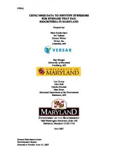
length of ∼175 kb. Interestingly, methods based on SNP chips generate widely varying estimates, ranging from 7.5 kb to 200 kb. Some of this variability seems to be explained by differences between the genotyping platforms and the resolution of the algorithms used to analyze the data. As more recent experimental methods yield much shorter estimates of median CNV length (even though they should be well powered to detect longer CNVs), it seems likely that the CNV lengths reported from BAC CGH arrays and some genotyping arrays are overestimates [56]. Origin of CNVs Fig. 1. Median CNV length for 23 studies in the Database of Genomic Variants. After excluding polymorphisms 100 kb in length, duplications are more frequent than deletions [20]. The DGV contains CNVs as large as 8 Mb, with a median size of 17.6 kb. The inferred length of a detected CNV is dependent on aspects of the underlying technology, such as probe spacing, probe length and signal resolution. To illustrate the differences between technologies, we calculated the median CNV length for all studies collected in the DGV (Figure 1), excluding variants shorter than 1 kb. The median length of detected CNVs varies a great deal across studies, and the distribution of CNV length suggests that BAC arrays and ROMA tend to overestimate CNV size. Among studies that report at least 50 CNVs, the longest observed median CNV length is 225 kb [43], while the shortest observed median CNV length is 2.5 kb [26]. The median length of a study is clearly dependent on its method of CNV detection. Agilent CGH methods, sequencing and methods based on Mendelian inconsistencies estimate a median length of ∼10 kb, while methods based on BAC CGH and ROMA suggest a median
While CNVs are ubiquitous throughout the genome, we have only limited understanding of their mutation process. The high frequency of CNVs in regions of segmental duplication suggests that these CNVs are generated by nonallelic homologous recombination [54]. By careful analysis of the flanking sequence of 98 insertions and 129 deletions, Kidd et al. [24] determined that about 40% of those CNVs were caused by nonallelic homologous recombination. Of the remaining insertions, ∼30% were caused by nonhomologous end joining, ∼20% by retrotransposition and ∼10% by expansion or contraction of a variable number of tandem repeats. Among deletions, ∼45% were caused by nonhomologous end joining and ∼15% by retrotransposition, while a variable number of tandem repeat regions did not contribute. These distributions depended on the size of the CNV; the proportion of CNVs formed by nonallelic homologous recombination is larger among CNVs > 5 kb. In a recent study, Arlt et al. [1] subjected human fibroblasts to mitotic replication stress, which resulted in numerous copy number changes. The authors observed that most breakpoint junctions showed micro-homologies, suggesting that the copy number changes were generated by nonhomologous end joining. It is not yet clear if the same processes generate naturally occurring CNVs. Further work is necessary to estimate the rates of these events and to understand the contribution of surrounding genetic motifs. Such understanding may allow us to predict mutation hotspots for CNV and to estimate mutation rates at these locations. Based on these parameters, we can design methods to infer the location of CNVs and hotspots of de novo mutations. In fact, several studies have used features of genomic DNA such as segmental duplications to predict the locations of CNVs [47, 48].
4
¨ S. ZOLLNER AND T. M. TESLOVICH
Current estimates of the rates of de novo CNV mutations derive from family studies. CNV status is inferred for members of a nuclear family, and CNVs observed in the offspring, but not in the parents, are assumed to be de novo variants. As both false positives in the offspring and false negatives in the parents result in false inference of a de novo event, it seems likely that the high rates of de novo events reported in some publications may be the result of cell line artifacts or affected by the high error rates of the applied CNV detection methods. In a recent study that carefully controlled for such errors, McCarroll et al. [35] observed 10 de novo events in 60 families, suggesting de novo mutation rates of ∼0.08 per generation per genome. When assessing de novo CNV mutation directly by sperm typing, Turner et al. [53] estimated rates between 5 · 10−5 and 9 · 10−7 per genome per generation at four likely CNV mutation hotspots selected for their high rates of nonallelic homologous recombination. Rates of de novo CNV mutation also are reflected in the extent of linkage disequilibrium (LD) between CNVs and flanking markers. If a CNV arises once during evolution, the LD pattern observed between the CNV and nearby SNPs is expected to resemble the pattern of LD observed between pairs of SNPs. On the other hand, if multiple mutational events generate apparently identical CNVs, and each mutation event occurs on a different haplotype background, we expect to observe little or no LD between the CNV and adjacent markers. Several studies have suggested that the extent of LD between CNVs and markers is comparable to the LD between pairs of SNPs [15, 35], implying a low de novo mutation rate of CNVs. CNVs in segmental duplications are reported to have less LD with nearby SNPs [28]. It is unclear whether this reduced LD is truly caused by a higher rate of CNV mutation in these regions, or whether this observation is an artifact of reduced SNP coverage. As SNP density in segmental duplications is generally lower than in other genomic regions due to the difficulty of designing high-quality genotyping assays for duplicated SNPs [28], marker panels are less likely to contain markers with the allele frequency necessary to obtain high values of r 2 . Nevertheless, coalescent simulations show that even relatively high mutation rates of 10−5 are consistent with high levels of linkage disequilibrium [61]. Frequency Spectrum and Signals of Selection Mutation rates of some CNVs are several orders of magnitude higher than mutation rates of SNPs
[36]; therefore, it is remarkable that CNVs show an excess of rare variants, compared to population genetic predictions [5]. Recently, Itsara et al. [20] reported that in a sample of 2500 individuals, 35% of all copy number variable sequence was copy number variable in a single individual. Less than 1% of CNVs had MAF > 1%. McCarroll et al. [35] reported after analyzing the HapMap sample that only 38% of detected CNVs had MAF > 1%. The same paper [35] emphasizes that 8% of CNVs responsible for interindividual variability have MAF ≤ 1%. This estimate is again consistent with an excess of rare variants; population genetics models of constant population size predict that 2% of mean difference between individuals will be generated by polymorphisms with MAF ≤ 1%. Nevertheless, CNVs with appreciable MAF occur worldwide. Jakobsson et al. [21] explored the distribution of 396 nonsingleton CNV loci inferred in a worldwide sample of 405 individuals from 29 populations, observing that 69% of the detected CNVs occurred in more than one continental group. Using the CNVs to form a population history, they recaptured the same evolutionary history that is inferred from SNP data. In comparison, Kidd et al. [24] reported that of 1695 CNVs detected in a panel of four Yoruba, two CEPH, one Chinese and one Japanese individual, 15% of all CNVs were observed in two or more continental groups. When analyzing the HapMap sample using the Affymetrix 6.0 chip, McCarroll et al. [35] found that 42% of all nonsingleton CNVs were present in more than one continental group. While the differences between these estimates may be a result of the different experimental platforms used, the common message is that a large proportion of common CNVs can be found worldwide. Whether this wide dispersal of common CNVs is the result of parallel mutation in multiple ethnic groups or migration is not clear. The frequency distribution of CNVs, with its strong excess of rare variants, can be interpreted as a signal of purifying selection acting on CNV loci, or as a signal of population growth. Under a model of population growth we would observe similar allele frequency distributions for CNVs and SNPs, as both are subject to the same history. However, we observe a greater excess of rare variants among CNVs than among SNPs, indicating that purifying selection is acting to remove many derived CNV alleles from the population [5, 43]. This theory is further supported by the finding that rare CNVs are more likely to
COPY NUMBER VARIANTS
5
statistical association and biological understanding is complicated by the fact that even CNVs that duplicate or delete entire genes may not result in discernable phenotypes. Moreover, which genes are affected by a CNV may be hard to predict. Recent studies comparing gene expression and CNVs across twelve inbred strains of mice demonstrated that, other than in the CCL3L1 gene, changes in copy number often have little or no effect on expression levels [14]. On the other hand, the same study showed that longer CNVs can alter the expression of genes over a distance of up to 3 Mb. Thus, CNVs that contribute to disease risk may do so by acting on causal genes not normally associated with the location of the CNV, creating yet another challenge Functional Signals of CNVs as we seek to understand the molecular mechanisms Given these signals for purifying selection, it is underlying disease risk. unsurprising that several CNVs affecting the risk A final challenge of detecting CNVs affecting comof common complex disorders have been reported. mon disorders is the small effect size of such CNVs. Widely cited is the effect on HIV/AIDS risk of a Given prior genetic epidemiology experiences with copy number polymorphism encompassing the gene common complex diseases, we can make predictions encoding CCL3L1 [13], a potent human immunode- about possible effect sizes of CNVs under different ficiency virus-1 (HIV-1)—suppressive chemokine and scenarios. Consider a common CNV (MAF > 5%) ligand for the HIV co-receptor CCR5. Lower copy that is tagged by surrounding SNPs. If such a CNV number of the CCL3L1 gene results in reduced se- had a large effect size (OR > 2), the surrounding cretion of the CCL3L1 protein and is associated with SNPs would present a strong signal for association increased risk of HIV-1 infection. More recently, re- in a GWAS, and the region would easily be identiduced copy number of the beta-defensin gene cluster fied. So far, no such CNV has been detected; CNVs has been reported to be associated with susceptibil- detected through LD with neighboring SNPs have ity to infectious and inflammatory diseases, particu- small effect sizes, comparable to those of diseaselarly Crohn’s disease [11, 34] and psoriasis [16]. Fur- associated SNPs [34, 59]. thermore, results of Willer et al. [59] implicated a 45 Rare CNVs that segregate in the population are kb deletion upstream of NEGR1 as being associated transmitted to offspring according to Mendel’s rules. with body-mass index. Hence, CNVs with effect sizes comparable to those As most CNVs are rare, it can be difficult to demon- of variants underlying Mendelian disorders are exstrate a statistically significant association between pected to generate strong linkage signals. However, a specific allele and disease. Hence, some studies for the last 30 years, geneticists have collected famhave examined the association between disease sta- ilies for common complex disorders and failed to tus and total CNV load. Rather than testing for as- identify linkage signals that can be explained by sociation between a single CNV and a disease phe- CNV. The absence of strong linkage and associanotype, such analyses assess whether cases have a tion signals indicates that there is an upper bound significant excess of CNVs (either deletions or inser- on the effect size of inherited CNVs that contribute tions) compared to controls. Using this design, Sebat to complex traits. Population samples are unlikely et al. [44] demonstrated a contribution of deletions to discover inherited CNVs with large effect sizes. to the risk of autism. More recently, Walsh et al. [55] reported that de novo insertions contribute to the IDENTIFYING CNVS IN GWAS risk of schizophrenia, and Zhang et al. [60] presented Given their genomic patterns, CNVs are enticing similar results for bipolar disorder. While several risk-CNVs have been detected, the candidates for causative variants, and it is of great mechanisms by which these CNVs increase disease interest to identify CNVs associated with common risk are largely unknown. Bridging the gap between diseases. As many CNVs are rare, and the effect sizes
overlap with genes than common CNVs [20]. Similar evidence has been observed in model organisms: In inbred mouse strains, Henrichsen et al. [14] reported a paucity of CNVs in ubiquitously expressed household genes and an excess of CNVs in genes with highly variable or tissue-specific expression patterns as evidence that CNVs are under purifying selection. Moreover, Emerson et al. [10] reported evidence that standing copy number variation in Drosophila is reduced due to purifying selection. As the selection acting on CNVs is more pronounced than that observed for SNPs, CNVs are likely to have greater functional impact than SNPs, negatively affecting the reproductive fitness of carriers.
6
¨ S. ZOLLNER AND T. M. TESLOVICH
of common CNVs are likely to be small, such studies require large sample sizes. Genome-wide association studies that type densely spaced panels of SNPs in large samples of cases and controls are already commonplace, and therefore provide an inexpensive resource to explore the contribution of CNVs to common diseases. The utility of this approach depends on how many CNVs are covered by the probes on genotyping arrays. Older genotyping arrays type relatively few SNPs within common CNVs. As markers located within CNVs are likely to fail multiple quality control criteria such as HWE, early array designs excluded such “problematic” markers. Newer genotyping technologies such as the Affymetrix 6.0 and the Illumina Human1M-Duo BeadChip have increased coverage of CNV regions. Even most of the arrays commonly used today directly interrogate only a subset of known CNVs. McCarroll et al. [35] reported that only 44% of common CNVs detected in HapMap samples were represented by at least one SNP on the Affymetrix 500K or Illumina 650Y arrays, and less than 20% of common CNVs are represented by three or more SNPs. It has been estimated that at least 20% of deletions longer than 1 kb span exactly zero probes on all commercially available arrays [6]. As accurate copy number estimates require typing multiple SNPs within a CNV, the ability to infer CNVs directly is limited by this coverage. Most modern genotyping chips contain dedicated CNV probes to facilitate copy number estimation. The Affymetrix 6.0 chip contains 800,000 probes equally spaced over the genome, as well as 140,000 probes targeted specifically at known CNV regions [35]; the Illumina Human1M-Duo BeadChip contains 36,000 nonpolymorphic probes to interrogate known CNV regions. During analysis, such CNV probes can either be analyzed individually or combined with SNP probes by treating CNV probes as genotyping probes covering monomorphic SNPs. Independent of the specific platform, several challenges must be overcome to perform thorough copy number analysis using GWAS data. First, the signal is sparse; >99% of each individual genome is at normal copy number compared to a reference sequence. Second, the signal is noisy, and a single SNP or probe is usually insufficient to predict copy number status. At least three types of evidence have been extracted from genotyping data and used to infer the presence of CNVs: (1) Non-Mendelian Inheritance
errors (NMIs) in family data; (2) Departures from Hardy–Weinberg Equilibrium (HWE); and (3) Differences in signal intensity measured during the genotyping reaction. Non-Mendelian Inheritance Errors (NMIs) in Family Data Deletions segregating in families can cause the appearance of non-Mendelian inheritance; hence, NMI analysis has proven to be a powerful approach to localize deletions [5, 33]. In most genotyping assays, hemizygous genotypes are inferred to be homozygous for the present allele. If a hemizygous parent transmits the deletion-carrying chromosome during meiosis, the child will be hemizygous and appear to be homozygous for the allele transmitted from the other parent. If that allele is different from the allele observed in the parent transmitting the deletion, the offspring’s genotype will be inconsistent with his two parents under Mendel’s rules, and the trio will be considered to be an NMI (Figure 2). The observation of multiple consecutive SNPs with non-Mendelian inheritance in the same trio indicates the presence of a segregating deletion. However, not all deletions can be identified through NMI analysis. Carriers in the parental generation will be identified only if the chromosome carrying the deletion is transmitted to the offspring. Even a transmitted deletion will generate an NMI only if the allele transmitted from the other parent is inconsistent. The probability of the deletion being transmitted is 0.5 and the probability of a transmitted deletion creating an NMI is equal to the heterozygosity of the SNP. Thus, the probability of observing an NMI if one of the parents carries a deletion is equal to half the heterozygosity of the SNP, therefore ≤0.25. Since consecutive SNPs covered by a deletion are usually in LD, they do not generate NMIs independently of one another even when conditioning on the deletion being transmitted. Hence, the probability of seeing any pattern of NMIs among consecutive SNPs depends on the haplotype frequencies in the population. Departures from the Hardy–Weinberg Equilibrium Not only will genotyping algorithms generally identify hemizygous individuals as homozygotes, they also will call homozygous SNPs in duplicated regions as heterozygous, if different alleles are present at the two different loci. Consequently, observed genotype
COPY NUMBER VARIANTS
7
Differences in Signal Intensity Measured During the Genotyping Reaction
Fig. 2. Mendelian inheritance errors. The left panel displays the genotype of a nuclear family at a single marker; the father is hemizygous for a deletion that has been transmitted to the offspring. The right panel shows the genotypes as they would be called by a genotyping algorithm. Both hemizygotes are falsely typed as homozygotes. Note that even though the actual transmission in the right panel follows Mendel’s rules, the observed genotypes seem to indicate an impossible inheritance.
frequencies of SNPs covered by deletions or duplications may show departures from HWE. SNPs within a deletion will show an excess of homozygous genotypes for both alleles. Consecutive SNPs all showing an excess of homozygote calls are indicators of a segregating deletion, and the minor allele frequencies of SNPs within a deletion will be overestimated from the data. The expected excess of homozygotes can be expressed dependent on the frequency of the deletion, and the deletion frequency can be estimated from the difference between the expected and the observed number of homozygotes (see the Appendix for details). For SNPs covered by duplications, the scenario is more complicated. SNPs within a duplication usually will show an excess of heterozygous genotype calls; the magnitude of this excess depends on the frequency of the duplication, the distribution of alleles that have been duplicated and the LD between the original region and the duplicate(s). Hence, the frequency of a duplication cannot be estimated from genotyping data. In the Appendix, we provide an overview of the change in genotype and allele frequencies generated by this effect. Note that such considerations assume uniform behavior of genotyping algorithms. For some SNPs within a duplication, genotype clustering algorithms may not be able to assign the correct three clusters to the intensity signal, and produce false genotype calls or fail to call the SNP. Thus, markers that fail quality control should be examined carefully to determine whether they lie within CNVs.
Last, we can use the intermediate signal generated by modern genotyping platforms to infer CNVs. The two most commonly used high-throughput genotyping platforms (Illumina and Affymetrix) genotype by hybridizing the DNA of an individual to a chip, generating a fluorescent signal for each allele at every marker tested. The intensity of this fluorescent signal depends on the number of alleles present. Due to the dynamic range of modern arrays, which have been optimized to yield accurate genotype calls, and since the scanners used to detect signal become saturated, hybridization intensity is not quite proportional to the number of copies of an allele. Moreover, the intensity distribution varies between probes and between genotypes for each probe [62]. Consequently, it is not obvious how to model the distribution of hybridization intensities. The intensity of the signal also depends on all of the usual confounders of oligonucleotide array analysis such as the total amount of DNA hybridized, background fluorescence and hybridization quality [9, 37]. The signal distribution along a chromosome has been described to show a wave-like pattern easily mistaken for CNVs [31]. Finally, interpreting this signal is challenging because the inference of CNV status is confounded with the genotype calling based on the same signal. Especially for low-quality DNA data (e.g., from whole genome amplification), hybridization intensities are often unsuitable to call CNVs although SNP genotype calls may be accurate [41]. An important first step in the analysis of hybridization data is the normalization of signal intensities. The raw data usually will consist of one intensity signal for each of the two possible alleles. The goal of the normalization step is to transform the two dimensional data into a single random variable that is identically distributed for all loci with baseline copy number, independent of the underlying genotype. For Illumina arrays, this normalization is usually performed by calculating the Log-R ratio. The calculation involves outlier removal, followed by normalization against background signal. Based on these normalized intensities, genotypes are called. The LogR ratio (LRR) is the logarithm of the ratio of the observed signal for a particular individual to the average signal of individuals in the reference panel with the same genotype. Hence, individuals with the same copy number as those in the reference panel
8
¨ S. ZOLLNER AND T. M. TESLOVICH
have LRR ≈ 0, while LRR < 0 indicates a deletion, and LRR > 0 indicates duplication. This normalization algorithm assumes that individuals in the reference panel have the baseline copy number for all markers. If this is not the case, the normalization will be shifted, a problem, especially, for individuals carrying rare alleles [62]. In addition, Illumina’s normalization procedure provides the B allele frequency (BAF), a measure for the ratio of intensity signals between the two genotyping channels. This statistic can be considered to be a quantitative representation of genotype, taking values near 0 or 1 for homozygous genotypes and near 0.5 for heterozygous genotypes. For Affymetrix arrays, no equivalent widely-used normalization strategy exists. While quantile methods are most often used to normalize the overall hybridization intensity across arrays (e.g., [23]), most methods analyzing Affymetrix data employ additional, method-specific normalization algorithms to account for differences in hybridization intensity distribution between loci and alleles. EXISTING METHODS FOR ANALYZING GWAS DATA Two possible strategies exist for analyzing the contribution of CNVs to common diseases in GWAS data. Either CNVs are tested using nearby SNPs as proxies, or CNVs are inferred from genotyping data, and the resulting calls are tested for association. Linkage Disequilibrium (LD) Between CNVs and Nearby SNPs As common CNVs in unique regions of the genome are often in strong LD with neighboring SNPs [15, 35], these SNPs serve as proxies for the linked CNVs, and SNP genotyping is an accurate and inexpensive alternative to CNV typing. The utility of a SNP as a proxy measure is dependent on the r 2 between the SNP and the CNV. For CNVs typed in the HapMap sample [35] and other large population samples [20], it is possible to define a set of CNVs that are well tagged by known markers. McCarroll et al. [35] reported that most common (MAF > 5%), biallelic CNVs discovered in HapMap samples can be captured perfectly by at least one SNP in the HapMap Phase II data (r 2 = 1 between CNV and tag SNP); however, only 30–40% of these CNVs are tagged perfectly by SNPs on commercially available genotyping arrays, while 45–65% can be captured by
markers with r 2 > 0.8. Similarly, Cooper et al. [6] reported that, among 84 common deletions observed in eight Yoruba, Japanese, Chinese and CEPH samples (worldwide MAF > 5%), 82% were tagged by at least one HapMap Phase II SNP with r 2 > 0.8, and 48–54% were captured (r 2 > 0.8) by markers on commercially available arrays. As standard operating procedure, GWAS impute all HapMap markers, using algorithms such as MACH [27], and test them for association. Consequently, GWAS studies already test SNPs tagging most common CNVs. This strategy has been used successfully to identify CNVs associated with complex traits [34, 59]. However, this strategy has some weaknesses: First, tag SNPs cannot be used to infer rare CNV alleles or de novo events. Second, since most markers on commercial arrays are biallelic, multiallelic CNVs are necessarily poorly tagged. Third, CNVs located in segmental duplications are generally more difficult to tag [35, 46]. For these reasons, the copy number status of many CNVs must be estimated using other methods. Analyzing CNV Calls Early approaches for identifying CNVs from genotyping data focused largely on NMIs and departures from HWE to identify deletions in HapMap samples [5, 33]. Kohler and Cutler [22] combined NMIs, deviations from HWE and frequency of missing data to infer deletions from GWAS data. Presently, most CNV detection methods focus on analyzing hybridization intensity data, often ignoring other sources of information such as LD or departure from HWE. To identify CNVs, researchers adapted several methods that were originally designed to analyze cancer data (e.g., circular binary segmentation, CBS [38]) or designed for other platforms. The first method specifically designed for genotyping arrays is an extension of the SW-ARRAY algorithm [39] by Komura et al. [25] to analyze data from Affymetrix 500K chips. In the recent literature, hidden Markov model (HMM) methods are the most commonly applied tool. First proposed by Fridlyand et al. [12], these methods exploit the local correlation of trait status. As CNVs often extend over multiple markers, combining information across neighboring markers is often more powerful than looking at one marker at a time. Colella et al. [4] proposed an objective Bayes Hidden Markov Model to infer location and carrier status of CNVs from Illumina BeadArray data. With PennCNV [56], Wang et al.
9
COPY NUMBER VARIANTS
extended this model to utilize information for related individuals. Such HMM methods have been applied in many projects (i.e., [20, 21]), and most CNVs in the databases have been located with these or similar algorithms. Unfortunately, HMM methods have relatively high error rates, especially for shorter CNVs. PennCNV has an error rate of 25% for CNVs of any length and 9% for CNVs encompassing ten or more SNPs [56]. While no error rates have been reported for other HMM methods, they are not fundamentally different from PennCNV and, it is unlikely that they perform substantially better. Most HMM and CBS methods used to infer CNVs analyze one individual at a time, and only posthoc combine the calls across individuals. While this keeps the memory requirements for each analysis to a minimum, it potentially reduces the ability to exploit occurrences of the same CNV in multiple individuals. Recently, methods designed under a different paradigm have been published. Rather than scanning the genome for signals of copy number variation, these methods only analyze known copynumber variable regions. Such methods do not have to account for the uncertainty of the CNV location, and can therefore generate more precise estimates of carrier status. The algorithm Canary [23] fits a Gaussian Mixture model to the intensity distribution and assigns copy number status according to cluster membership. Other recent methods attempt to quantify the uncertainty of the CNV call; such measures of uncertainty can be incorporated into tests for association by weighting each call according to its confidence. CNVEM [62] is based on a similar idea, using a Bayesian framework to calculate the posterior probability of copy number, thus accounting for the uncertainty in the CNV genotyping. Similarly, Barnes et al. [2] proposed a frequentist method of modeling copy number states as a latent variable and then using a mixture model to test for association. All of the methods focusing on known CNVs report substantially lower error rates compared to HMM models, although few such estimates of error rates have been replicated independently. Such methods for calling known CNVs depend on precise estimates of CNV location. Large collections of CNVs have been described in multiple databases, including the Database of Genomic Variants (DGV) [8], the Human Genome Structural Variation Project [18] and the Copy Number Variation Project Data Index [7]. Some care must be taken
when selecting loci from these databases; as technology and algorithms used to detect CNV are still evolving, these databases contain false positives, and not all common copy number variants have been detected and reported. Furthermore, the boundaries of CNVs in these databases may be imprecise, as some methods for CNV detection only yield approximate boundaries. In practice, it may be advisable to focus on CNV collections reported by recent studies, as these tend to be based on more precise methodology. Of course, focusing on CNVs reported in databases is not appropriate when exploring the impact of de novo CNV mutations, since such variants may not have been previously observed. In this case, the analysis can be performed in two steps, with an initial CNV discovery step using an HMM such as PennCNV. While such methods may not detect every CNV in each carrier, it is sufficient to identify each CNV once in the sample and to generate estimates of its borders. In a second step, the copy number status of these CNVs can be called in all individuals using more precise algorithms. Comparing Tag SNPs and CNV Calling It is not obvious whether directly estimating CNV carrier status is actually a useful strategy if a CNV is tagged by nearby SNPs; even in the best case, methods estimating the carrier status of a CNV have much higher error rates than SNP genotyping [23]. The answer depends on the degree of LD between the CNV and the proxy SNPs, as well as the error rate for inferring CNVs directly. Here we assess which approach is more powerful, by determining the sample size inflation necessary to overcome power loss due to errors in CNV inferences, and compare it to the inflation in sample size necessary to overcome the power loss due to incomplete LD (r 2 < 1). We show that under many scenarios, testing tag SNPs results in a more powerful test than calling CNVs and testing inferred CNV calls. Following an argument from Pritchard and Przeworski [40], we derive the distribution of a χ2 -test for association based on a 2×2 contingency table dependent on the rate of calling error. Based on that distribution, we calculate the inflation factor (IF ) by which the sample size needs to be increased to overcome the loss of power due to CNV calling errors. Assuming no calling error, the distribution of a χ2 -test in a sample of N1 cases and N1 controls is χ21 =
(P (C|case) − P (C|control ))2 N1 , 2P (C)(1 − P (C))
¨ S. ZOLLNER AND T. M. TESLOVICH
10
where P (C|case) is the observed frequency of the minor CNV allele in cases, P (C|control ) is the observed frequency of the minor CNV allele in controls and P (C) is the overall observed frequency of the minor CNV allele. Now let O be the event of calling the minor allele of the CNV, C the event of the minor CNV allele being present and A the event of the major CNV allele being present. Then we can parameterize P (O|C) as the probability of correctly calling the minor allele if the minor allele is present and P (O|A) as the probability of falsely calling the minor allele if the major allele is present. Hence, P (O) = P (O|C)P (C) + P (O|A)P (A) is the total number of CNVs being called in the sample. In this model, the χ2 -test for association in a sample of N2 cases and N2 controls is χ22 = ([P (O|C) − P (O|A)] × [P (C|case) − P (C|control )])2 N2 /(2P (O)(1 − P (O))). To calculate the increase in sample size necessary to overcome the loss of power due to errors in calling CNV alleles, we can calculate the inflation factor (IF ): IF =
P (O)(1 − P (O)) 1 N2 = . 2 N1 (P (O|C) − P (O|A)) P (C)(1 − P (C))
The right side of the equation indicates the factor by which the sample size has to be multiplied to overcome the loss of power due to calling errors. This inflation factor can be directly compared to the inflation of sample size necessary to overcome incomplete LD (r 2 < 1), as testing for association at a marker with r 2 = x to the risk variant inflates the sample size by 1/x [40]. To compare tagging strategies with direct calling of CNVs, we calculated the inflation factor for a range of error rates and CNV frequencies commonly reported in the literature (Table 1). Most CNV calling methods have reported error rates between 0.1 and 0.3. As falsely calling the rare allele of a CNV at a specific location is unlikely under most methods, we assumed that most errors were false calls of the major allele in the presence of the minor allele; the probability of such errors is (1 − P (O|C)); we consider values of P (O|C) between 0.7 and 0.9, for values of P (O|A) of 0.01 and 0.05. For larger values of P (O|A), the inflation factor increases rapidly (data not shown). For comparison, we also calculated the
r 2 between the CNV and the best tag SNP that results in the same inflation factor for the tag SNP approach. Our results indicate that calling error reduces the power of testing rare CNVs more than it reduces the power of testing common CNVs. Even modest error rates [P (O|A) = 0.01, P (O|C) = 0.8] increase the required sample size for finding rare CNVs (MAF = 0.02) by 50% or more, particularly relevant as large sample sizes are required to detect these rare variants in the first place (Table 1). Comparison with LD statistics indicates that, under these conditions, a SNP tagging the CNV with r 2 ≥ 0.49 is sufficient to provide a more powerful test than inferring CNV status and directly testing the CNV for association with disease. Furthermore, a high false positive rate [P (O|A)] increases the sample size more than does a high false negative rate (1 − P (O|C)). For high values of P (O|A), inferring and testing a CNV yields poor results, compared to the tagging method; under all considered parameter combinations, a tag SNP with r 2 ≥ 0.67 to the CNV allows for a more powerful test for association. Note that these considerations assume that only a single tag SNP provides information about the allelic state of the CNV. In practice, we can expect multiple SNPs to be in LD with the CNV, and combining information across tag SNPs will result in an even more powerful test statistic. However, when no tag SNP is available for a particular CNV, valuable information may be gained by inferring CNV status directly from GWAS data. TESTING CNVS FOR ASSOCIATION WITH DISEASE After inferring carrier status, several methods can be used to test for association between inferred carrier status and disease. As most CNVs are biallelic, we can apply methods developed for rejecting the null hypothesis of no association between a biallelic marker and a phenotype, such as the chi-square test or logistic regression. In such studies we consider the inferred carrier status to be the true carrier status. However, in tests for transmission distortion [17, 50] it should be considered that transmitted CNVs are generally easier to detect than nontransmitted CNVs, particularly if NMIs are used to identify carriers. A further potential problem may be generated by the stringency of the CNV calling algorithm. Commonly, such algorithms impose
11
COPY NUMBER VARIANTS
Table 1 Impact of calling error on association testing for common CNVs. We display the inflation factor (IF ) for sample size, necessary to overcome typing error of common CNVs. The first line shows the sample frequency of the rare CNV allele, the first column shows the probability of falsely calling the rare CNV allele and the second column shows the probability of correctly calling the rare CNV allele. For each set of parameters the table shows the inflation factor (IF ) for the sample size to overcome the effects of this genotyping error and the LD (r 2 ) to a tag SNP that results in the same loss of power P (C) (freq. of minor CNV allele) P (O|A)
P (O|C)
(false positive rate)
0.02
0.05
(sensitivity)
IF
r
0.01
0.9 0.8 0.7
1.74 2.05 2.49
0.05
0.9 0.8 0.7
4.41 5.51 7.13
2
0.1
IF
r
0.57 0.49 0.40
1.37 1.59 1.88
0.23 0.18 0.14
2.45 2.99 3.77
a high burden of proof (e.g., posterior probability > 0.95) before assigning the minor allele, in order to minimize the effects of measurement error. This approach can increase the number of false negative calls and introduce nonrandom missingness, thus inflating the false-positive rate of a family-based test for association [2]. Tests for association can be improved by accounting for the uncertainty in the estimate of carrier status. Bayesian methods will generally provide a posterior probability for carrier status [2, 62], and in frequentist inference methods this uncertainty can be ascertained by bootstrap or jackknife procedures. Once this uncertainty is known, tests for association can be adjusted accordingly. For Bayesian estimates we can compare the summed expected posterior carrier status in a χ2 test or in a logistic expression. Finally, Stranger et al. [52] skip the step of inferring CNV status for such regions and directly test for association between hybridization intensity and case-control status. This method is susceptible to false positives due to shifts in mean and/or variance of the underlying intensity distributions, and such shifts occur frequently in practice [2]. ALTERNATIVE STRATEGIES TO ASSOCIATION MAPPING As most CNVs have low MAF, tests for association between a single CNV and a disease are likely to have low power, especially if p-values are corrected for multiple tests. Therefore, alternative strategies must be considered. Here we present two such strategies: first a test for an excess of de novo CNV mutations at a locus and second a test for an excess
2
0.2 IF
r2
0.80 0.69 0.59
1.20 1.40 1.66
0.83 0.71 0.60
0.56 0.46 0.37
1.48 1.78 2.18
0.67 0.56 0.46
IF
r
0.73 0.63 0.53
1.25 1.44 1.70
0.41 0.33 0.27
1.80 2.16 2.68
2
loading of minor CNV alleles in cases compared to controls. Detection of de novo CNVs As recent results indicate that de novo CNV mutations are rare [35], multiple de novo mutations in the same region of the genome suggest candidates for risk variants. However, even if de novo mutations are over-represented and highly penetrant among cases, the combined variants at one locus are still unlikely to have allele frequency > 1% in cases. Hence, applying standard testing strategies to compare allele frequencies between cases and controls will be underpowered. Consider, for example, a genomic region carrying 6 de novo mutations in 1000 cases, and none in 1000 controls. Testing for association yields a Fisher’s exact p-value of 0.015, no clear evidence of association. However, this p-value does not account for the observation that the rate of de novo mutations is low and therefore the probability of observing 6 de novo deletions at the same locus by chance is unlikely. Nevertheless, it is not clear how many de novo mutations must be observed in the same region before the finding is significant. Such a critical value depends on two parameters: the rate of de novo mutation, and the number of locations in the genome where such mutations occur. While the mutation rate can be estimated from existing data sets, early estimates of these rates were confounded with high false negative rates [57]. Recent studies suggest that these rates may be as low as 0.08 per genome per meiosis [35].
12
¨ S. ZOLLNER AND T. M. TESLOVICH
Estimating the second parameter, the number of genomic regions experiencing de novo CNV mutation, is more challenging. About 40% of CNVs are generated by nonallelic homologous recombination [24], which is caused by flanking repetitive elements and segmental duplications. Such segmental duplications cover 5% of the genome. Thus, it is likely that most nonpathogenic de novo mutations occur in only a small subset of the genome. However, better understanding of the processes generating CNVs are necessary for a precise estimate of the subset of the genome with high CNV mutation rate. To explore the power of detecting a risk variant by observing an excess of de novo mutations, we performed computer simulations based on the two parameters described above. We set the de novo mutation rate of noncausal CNVs to µ per meiosis per genome, uniformly distributed over k locations in the genome. We further assumed that a subset ε, of all de novo CNV alleles would be identified. We did not model other sources of error, as false positive de novo CNV calls, by definition, are not expected to cluster at particular loci in the genome, and therefore do not affect our test statistic. Assuming a sample of n nuclear families, we modeled as the null distribution the total number of detected noncausal de novo CNVs, ci , at each location i, as Poisson-distributed with rate 2µnε/k. Defining M = max{ci : i = 1, . . . , k} as the maximum number of noncausal de novo mutations observed anywhere in the genome, the critical value for a test of an excess of de novo CNVs is equal to CVα = min{x : P (M ≥ x) < α}. Note that the alpha level chosen here is the experiment-wide type I error rate; by maximizing M over all CNV mutation hotpots, we have corrected for genome-wide multiple testing. To simulate the distribution of causal de novo mutations at a risk locus, we set p as the proportion of cases in the population carrying the de novo CNV mutation at a specific risk locus. Then the power for a test of excess de novo mutations can be calculated using the binomial distribution, B(εp, n). We assessed the power of this method to detect a significant excess of de novo mutations. We first calculated critical values for sample sizes of n = 500, 1000 and 2000 nuclear families, assuming a de novo mutation rate of noncausal CNVs of µ = 0.1 per meiosis per genome, uniformly distributed over k = 500 or 2000 locations in the genome. Assuming an average length of 50 kb per CNV, these val-
ues of k correspond to 0.8% or 3.2% of the human genome being CNV mutation hotspots, with CNV mutation rates similar to the rates observed at hotspots of nonallelic homologous recombination [53]. We set an error rate for CNV typing of ε = 0.75. Based on the resulting critical values, we calculated the power of observing a significant result at α = 0.05, assuming that de novo CNVs occur in p = 1%, 0.5% or 0.25% of all cases at a particular risk locus. These values are consistent with reports that de novo CNVs thought to contribute to the risk of psychiatric diseases are observed in 0.2% to 1% of all cases [51, 53, 58]. For comparison, we calculated the total sample size necessary to achieve 80% power in a balanced case-control design at a significance level of 10−5 for all values of p, assuming that the CNV has full penetrance and is not observed among controls. Our results (Table 2) indicate that observing a large number of CNV mutations at a single locus is unlikely. Under all considered scenarios, observing 6 or more de novo CNVs at one locus constitutes a significant result. For sample sizes >1000 trios, we have reasonable power to detect de novo CNVs that are present in 0.5% of the cases. The results indicate that the power of this approach strongly depends on the total number of CNV mutation hotspots, which is unknown for the human genome. However, even if only 500 CNV hotspots exist genome-wide, for a CNV observed in 1% (0.5%) of all cases, only 1000 (2000) trios are necessary to achieve ∼80% power. For comparison, 5500 (11,000) unrelated individuals are required to achieve similar power. This suggests that testing for an excess of de novo mutations is a more powerful strategy than case-control testing. CNV Load of Rare Variants As discussed previously, most minor alleles of CNVs are rare, and tests of association between rare variants and a phenotype have limited power. However, it is conceivable that multiple, independent CNVs each contribute to disease risk. Jointly testing all CNVs may therefore be more powerful than testing markers individually. If all such risk CNVs cover the same genomic interval, the contribution of that region can be determined by counting the number of individuals who carry a minor allele of any CNV overlapping with the region. The counts in cases and controls can then be compared [32], essentially treating all overlapping CNVs as a single risk allele. Such joint analysis of multiple CNVs is more
13
COPY NUMBER VARIANTS
challenging under a model of genetic heterogeneity, which assumes that a large number of unlinked loci in the genome are affected by CNVs that contribute to the risk of disease. Under this model, testing each individual locus may not result in a significant signal. However, as the total number of CNVs in an apparently healthy individual is small [35], if several CNVs contribute to the risk of disease, cases as a whole may carry substantially more minor CNV alleles than do controls. Therefore, a commonly applied test is to count the number of minor CNV alleles observed genome-wide in cases, and compare that to the number of minor CNV alleles in controls. While such a test is more powerful under a model of genetic heterogeneity, it has two weaknesses. First, it is very sensitive to any experimental error affecting cases and controls differentially. For example, batch effects can increase the total number of CNVs observed in one batch over the next. If cases and controls are analyzed in different batches, such effects will immediately cause significant genome-wide differences in CNV numbers between cases and controls. Second, this test lacks interpretability. A significant signal only indicates that CNVs somewhere in the genome increase disease risk. Further testing of larger samples is required to understand the contribution of individual CNVs. CNVs that show an excess of minor alleles in cases that is not statistically significant may be good candidates for further tests in larger samples. This strategy has been used successfully to identify CNVs affecting autism. Initially, Sebat et al. [44] observed a genome-wide excess of CNVs in autism patients, but no individual CNV or locus was significant after multiple test correction. Further work
by Weiss et al. [58] in larger samples demonstrated that several of the loci showing suggestive evidence in the original report [44] are significantly associated with the risk of autism. CONCLUSIONS Copy number variation accounts for much of the genetic variation discovered to date in humans. Some of this variation is clearly functional; studies in recent years have discovered several CNVs contributing to the risk of common complex diseases such as autism [44] and psoriasis [16]. Hence, studying the contribution of CNVs to common diseases has become standard practice during the course of genomewide association studies. As the genotype and hybridization signals generated by genotyping platforms provide information about CNVs, it is efficient to use this signal to infer CNV location and carrier status in the sample. Most studies that impute CNVs from genotype array data focus on analyzing hybridization data. Such analyses require careful normalization of the intensity data, as hybridization signals are susceptible to experimental noise that may lead to false inferences. Many methods have been developed to localize CNVs using such hybridization intensity data (e.g., [25, 56]). While such methods generally perform well for CNVs covered by large numbers of probes, they tend to have higher error rates for CNVs that span only a few genotyped probes [56]. The high error rates are in part due to the fact that these methods aim to jointly localize CNVs and determine carrier status in individuals, thus increasing the uncertainty of the inference procedure. As databases now contain >20,000 CNVs, many of which have
Table 2 Critical values and power in tests for de novo mutations. The first row indicates the number of sites for noncausal CNVs, and the second line displays the sample size. The third line shows the number of CNVs in one location constituting a significant number of de novo CNVs. The next three lines show the power to detect a locus carrying an excess of de novo mutation, assuming that these de novo mutations can be observed in 1%, 0.5% or 0.25% of all cases. The last column provides the sample size necessary to detect the CNV with 80% power in a case-control design at a significance level of 10−5 Number of de novo CNV mutation hotspots 500
2000
Sample size
500
1000
2000
500
1000
2000
Case-control sample size
CVα 1.00% 0.50% 0.25%
4 0.52 0.12 0.02
5 0.86 0.32 0.04
6 >0.99 0.76 0.18
3 0.72 0.29 0.07
4 0.94 0.52 0.12
5 >0.99 0.94 0.52
5500 11,000 22,000
14
¨ S. ZOLLNER AND T. M. TESLOVICH
been observed more than once in different samples, it seems likely that most common CNVs are now known and that CNVs not yet present in databases are rare, at least in Caucasians. Consequently, algorithms have been developed that, using GWAS data, infer copy number for CNVs whose boundaries are known [23, 62]. Such algorithms are more precise in calling common CNVs and therefore facilitate more powerful tests for association. However, it is still necessary to apply more general algorithms to detect unknown CNVs, rare CNVs and de novo events. Most CNVs are in strong LD with SNPs in the HapMap, and it is not always clear that inferring CNVs to test for association is the most powerful strategy. As we have shown, even modest error rates in CNV calling result in a loss of power comparable to testing a tag SNP with r 2 ≤ 0.8. Consequently, tests based on inferred CNV alleles are often unlikely to be more powerful than testing surrounding SNPs for association. In this context, it is interesting to note that both common risk CNVs identified to date through genotype scans were first localized via tag SNPs; only follow-up testing identified these CNVs as likely risk alleles [34, 59]. On the other hand, this observation also indicates that SNPs flanking a CNV can provide information about CNV carrier status, suggesting that existing methods for calling CNV alleles could be improved by jointly considering haplotype background and hybridization intensity of the covered markers. As haplotype background and hybridization intensity provide orthogonal evidence for CNV status, such a method would likely be substantially more precise and allow more powerful tests. Maximizing the power of tests for association is crucial, as the effect sizes of common CNVs are likely to be small, and the minor alleles of most CNVs are rare. Hence, tests for association between CNVs and diseases are likely to have low power even under the best circumstances. Other strategies to identify CNV contributing to the risk of common diseases should also be explored. Recent studies have indicated that de novo events generating new CNVs are rare [35]. This suggests that testing a genomic region for an excess of de novo CNVs is potentially a powerful strategy. Moreover, such de novo CNVs are more likely to have large effect sizes. Several such CNV regions have in fact been detected [44, 55]. We have presented calculations, based on conservative estimates, that for moderate sample sizes, simple tests for local excesses of de novo mutations
have good power to identify such CNV mutation hotspots. However, commonly collected samples of unrelated cases and controls do not provide any information as to whether a CNV observed several times among cases and not in controls is the result of several de novo mutations or just a result of sampling variation on a rare CNV. Hence, the power to detect a rare risk variant that is the result of multiple de novo events is substantially higher in family-based studies. Any CNV-disease association identified using genotyping chips has to be evaluated carefully. While analyzing the hybridization signal from genotyping platforms provides cheap information about CNV status in a population, genotyping arrays are not the gold standard for determining carrier status. In association studies, erroneous calls of carrier status usually result in a loss of power, rather than false positive associations. However, in a study testing for an excess of de novo mutations, even a few inaccurate CNV calls can lead to false positives. Hence, if a CNV appears to be associated with a phenotype, it seems prudent to use an independent technology, such as CGH, PCR or resequencing, to verify the inferred carrier status and the association signal. In the near future, GWAS will be supplemented with studies that sequence regions of interest or even the entire genomes of affected and unaffected individuals. Paired end-sequencing allows the detection of regions where the distance between two short reads is significantly longer or shorter than expected; such regions are likely to carry CNVs. In the case of single-end sequencing, it is necessary to infer CNVs by indirect measures, such as the number of reads generated for each region. As read-lengths increase, it becomes easier to align reads, and it may become possible to identify CNV breakpoints within a read. Then it will be possible to identify such features from the generated sequence. As technology advances at an incredible pace, we will constantly be challenged to develop newer, better statistical tools to infer the presence and location of CNVs. Ultimately, to understand the role that CNV plays in human disease, we must better elucidate the biological processes that create CNV, improve the sensitivity and specificity of experimental methods that identify CNV, and develop statistical methods that fully leverage the signals of CNV that exist in data derived from genome-wide genotyping arrays as well as next-generation sequencing technologies.
15
COPY NUMBER VARIANTS
APPENDIX In the following we will explore patterns of genotype frequencies and the Hardy–Weinberg equilibrium in SNPs covered by CNVs. We consider the observed haplotype frequencies P (G = AA), P (G = AB), P (G = BB) of a SNP with alleles A and B. Let p be the population frequency of allele A and q the allele frequency of allele B. We first consider deletions, then duplications. Deletions We introduce the segregating deletion as a third genotype D with frequency d, so that d + p + q = 1. Let G ∈ {AA, BB, AB} indicate the possible observed genotypes and T ∈ {DD, AA, AD, AB, BD, BB} be the set of all possible true genotypes. Genotype DD will result in a failed genotyping reaction and hence will never be observed. Then, assuming no genotyping error for nondeletion alleles,
Insertions We consider a model where every haploid copy of the genome carries 0 or 1 insertions. Let T ∈ {A, B} indicate the true genotype at the original location and I ∈ {A, B} indicate the genotype at the duplication. To account for possible LD between the inserted region and the original copy, as insertions can happen multiple times, we consider the probability of carrying the insertion allele conditional on the allele at the original location, Q(I|T ). We define D ∈ {0, 1, 2}, the total number of insertions on both chromosomes, and the probability of carrying a duplication is dT : P (G = AA) = P (T = AA)[P (D = 0|A) + P (I = A)P (D = 1|A) + P (I = AA)P (D = 2|A)] 2
2
= p [(1 − dA ) + 2dA (1 − dA )Q(A|A)
P (G = AA) = P (T = AA|T 6= DD) + P (T = AD|T 6= DD) = (p2 + 2dp)/(1 − d2 ), P (G = BB) = P (T = BB|T 6= DD) + P (T = BD|T 6= DD) = (q 2 + 2dq)/(1 − d2 ), P (G = AB) = P (T = AB|T 6= DD) = 2pq/(1 − d2 ). Note that the estimated frequency of allele A is pest = P (G = AA) + 1/2P (G = AB) = (p + dp)/(1 − d2 ) = p/(1 − d), so that we will observe fewer than the expected number of heterozygotes, given the estimated allele frequencies: 2pest qest = 2pq/(1 − d)2 ≥ 2pq/(1 − d2 ) = E(G = AB). In a sample of n individuals with observed genotype counts (CAA , CAB , CBB ), the expected departure from HWE is E((CAB )2 − 4CAA CBB ) 2
= Var(CAB ) + E(CAB )
− 4[E(CAA )E(CBB ) + Cov(CAA , CBB )] = npq/(1 − d2 ) + 8ndpq(1 − n)/(1 − d).
+ d2A Q(A|A)2 ] = p2 (1 − dA Q(B|A))2 , P (G = BB) = q 2 (1 − dB Q(A|B))2 . Hence, P (G = AA) = P (T = AA) = p2 iff Q(A| A) = 1 or dA = 0. Similarly P (G = BB) = P (T = BB) = q 2 iff Q(B|B) = 1 or dB = 0. No departure from HWE is generated if all duplications with the A allele occur on chromosomes carrying the A allele at the original location (likewise for allele B), regardless of the frequency of the insertion. This pattern may be observed if duplications are the result of nonallelic homologous recombination or other mechanisms creating tandem repeats. ACKNOWLEDGMENTS We would like to thank Margit Burmeister, Don Conrad and Jun Li for thoughtful readings of the manuscript. SZ is supported by HL084729-02; TMT is supported by DK062370 and T32 HG00040. REFERENCES [1] Arlt, M. F., Mulle, J. G., Schaibley, V. M., Ragland, R. L., Durkin, S. G. et al. (2009). Replication stress induces genome-wide copy number changes in human cells that resemble polymorphic and pathogenic variants. Am. J. Hum. Genet. 84 339–350.
16
¨ S. ZOLLNER AND T. M. TESLOVICH
[2] Barnes, C., Plagnol, V., Fitzgerald, T., Redon, R., Marchini, J. et al. (2008). A robust statistical method for case-control association testing with copy number variation. Nat. Genet. 40 1245–1252. [3] Barrett, M. T., Scheffer, A., Ben-Dor, A., Sampas, N., Lipson, D. et al. (2004). Comparative genomic hybridization using oligonucleotide microarrays and total genomic DNA. Proc. Natl. Acad. Sci. USA 101 17765–17770. [4] Colella, S., Yau, C., Taylor, J. M., Mirza, G., Butler, H. et al. (2007). QuantiSNP: An Objective Bayes Hidden-Markov Model to detect and accurately map copy number variation using SNP genotyping data. Nucleic Acids Res. 35 2013–2025. [5] Conrad, D. F., Andrews, T. D., Carter, N. P., Hurles, M. E. and Pritchard, J. K. (2006). A high-resolution survey of deletion polymorphism in the human genome. Nat. Genet. 38 75–81. [6] Cooper, G. M., Zerr, T., Kidd, J. M., Eichler, E. E. and Nickerson, D. A. (2008). Systematic assessment of copy number variant detection via genome-wide SNP genotyping. Nat. Genet. 40 1199– 1203. [7] Copy Number Variation Project Data Index. http://www.sanger.ac.uk/humgen/cnv/. [8] Database of Genomic Variants. http:// projects.tcag.ca/variation/. [9] Eads, B., Cash, A., Bogart, K., Costello, J. and Andrews, J. (2006). Troubleshooting microarray hybridizations. Methods Enzymol. 411 34–49. [10] Emerson, J. J., Cardoso-Moreira, M., Borevitz, J. O. and Long, M. (2008). Natural selection shapes genome-wide patterns of copy-number polymorphism in Drosophila melanogaster. Science 320 1629–1631. [11] Fellermann, K., Stange, D. E., Schaeffeler, E., Schmalzl, H., Wehkamp, J. et al. (2006). A chromosome 8 gene-cluster polymorphism with low human beta-defensin 2 gene copy number predisposes to Crohn disease of the colon. Am. J. Hum. Genet. 79 439–448. [12] Fridlyand, J., Snijders, A. M., Pinkel, D., Albertson, D. G. and Jain, A. N. (2004). Hidden Markov models approach to the analysis of array CGH data. J. Multivariate Anal. 90 132–153. MR2064939 [13] Gonzalez, E., Kulkarni, H., Bolivar, H., Mangano, A., Sanchez, R. et al. (2005). The influence of CCL3L1 gene-containing segmental duplications on HIV-1/AIDS susceptibility. Science 307 1434–1440. [14] Henrichsen, C. N., Vinckenbosch, N., Zollner, S., Chaignat, E., Pradervand, S. et al. (2009). Segmental copy number variation shapes tissue transcriptomes. Nat. Genet. 41 424–429. [15] Hinds, D. A., Kloek, A. P., Jen, M., Chen, X. and Frazer, K. A. (2006). Common deletions and SNPs are in linkage disequilibrium in the human genome. Nat. Genet. 38 82–85. [16] Hollox, E. J., Huffmeier, U., Zeeuwen, P. L., Palla, R., Lascorz, J. et al. (2008). Psoriasis
[17]
[18] [19]
[20]
[21]
[22]
[23]
[24]
[25]
[26]
[27]
[28]
[29]
[30] [31]
is associated with increased beta-defensin genomic copy number. Nat. Genet. 40 23–25. Horvath, S., Xu, X. and Laird, N. M. (2001). The family based association test method: Strategies for studying general genotype–phenotype associations. Eur. J. Hum. Genet. 9 301–306. Human Genome Structural Variation Project. http://hgsv.washington.edu/. Iafrate, A. J., Feuk, L., Rivera, M. N., Listewnik, M. L., Donahoe, P. K. et al. (2004). Detection of large-scale variation in the human genome. Nat. Genet. 36 949–951. Itsara, A., Cooper, G. M., Baker, C., Girirajan, S., Li, J. et al. (2009). Population analysis of large copy number variants and hotspots of human genetic disease. Am. J. Hum. Genet. 84 148–161. Jakobsson, M., Scholz, S. W., Scheet, P., Gibbs, J. R., VanLiere, J. M. et al. (2008). Genotype, haplotype and copy-number variation in worldwide human populations. Nature 451 998– 1003. Kohler, J. R. and Cutler, D. J. (2007). Simultaneous discovery and testing of deletions for disease association in SNP genotyping studies. Am. J. Hum. Genet. 81 684–699. Korn, J. M., Kuruvilla, F. G., McCarroll, S. A., Wysoker, A., Nemesh, J. et al. (2008). Integrated genotype calling and association analysis of SNPs, common copy number polymorphisms and rare CNVs. Nat. Genet. 40 1253–1260. Kidd, J. M., Cooper, G. M., Donahue, W. F., Hayden, H. S., Sampas, N. et al. (2008). Mapping and sequencing of structural variation from eight human genomes. Nature 453 56–64. Komura, D., Shen, F., Ishikawa, S., Fitch, K. R., Chen, W. et al. (2006). Genome-wide detection of human copy number variations using high-density DNA oligonucleotide arrays. Genome Res. 16 1575– 1584. Levy, S., Sutton, G., Ng, P. C., Feuk, L., Halpern, A. L. et al. (2007). The diploid genome sequence of an individual human. PLoS Biol. 5 e254. Li, Y. and Abecasis, G. R. (2006). Mach 1.0: Rapid haplotype reconstruction and missing genotype inference. Am. J. Hum. Genet. S79 2290. Locke, D. P., Sharp, A. J., McCarroll, S. A., McGrath, S. D., Newman, T. L. et al. (2006). Linkage disequilibrium and heritability of copy-number polymorphisms within duplicated regions of the human genome. Am. J. Hum. Genet. 79 275–290. Lucito, R., Healy, J., Alexander, J., Reiner, A., Esposito, D. et al. (2003). Representational oligonucleotide microarray analysis: A highresolution method to detect genome copy number variation. Genome Res. 13 2291–2305. Maher, B. (2008). Personal genomes: The case of the missing heritability. Nature 456 18–21. Marioni, J. C., Thorne, N. P., Valsesia, A., Fitzgerald, T., Redon, R. et al. (2007). Breaking
COPY NUMBER VARIANTS
[32]
[33]
[34]
[35]
[36]
[37]
[38]
[39]
[40]
[41]
[42]
[43]
[44]
[45]
[46]
the waves: Improved detection of copy number variation from microarray-based comparative genomic hybridization. Genome Biol. 8 R228. McCarroll, S. A. (2008). Extending genome-wide association studies to copy-number variation. Hum. Mol. Genet. 17 R135–R142. McCarroll, S. A., Hadnott, T. N., Perry, G. H., Sabeti, P. C., Zody, M. C. et al. (2006). Common deletion polymorphisms in the human genome. Nat. Genet. 38 86–92. McCarroll, S. A., Huett, A., Kuballa, P., Chilewski, S. D., Landry, A. et al. (2008). Deletion polymorphism upstream of IRGM associated with altered IRGM expression and Crohn’s disease. Nat. Genet. 40 1107–1112. McCarroll, S. A., Kuruvilla, F. G., Korn, J. M., Cawley, S., Nemesh, J. et al. (2008). Integrated detection and population-genetic analysis of SNPs and copy number variation. Nat. Genet. 40 1166– 1174. Nachman, M. W. and Crowell, S. L. (2000). Estimate of the mutation rate per nucleotide in humans. Genetics 156 297–304. Nguyen, D. V., Arpat, A. B., Wang, N., Carroll, R. J. (2002). DNA microarray experiments: Biological and technological aspects. Biometrics 58 701–717. MR1939398 Olshen, A. B., Venkatraman, E. S., Lucito, R. and Wigler, M. (2004). Circular binary segmentation for the analysis of array-based DNA copy number data. Biostatistics 5 557–572. Price, T. S., Regan, R., Mott, R., Hedman, A., Honey, B. et al. (2005). SW-ARRAY: A dynamic programming solution for the identification of copynumber changes in genomic DNA using array comparative genome hybridization data. Nucleic Acids Res. 33 3455–3464. Pritchard, J. K. and Przeworski, M. (2001). Linkage disequilibrium in humans: Models and data. Am. J. Hum. Genet. 69 1–14. Pugh, T. J., Delaney, A. D., Farnoud, N., Flibotte, S., Griffith, M. et al. (2008). Impact of whole genome amplification on analysis of copy number variants. Nucleic Acids Res. 36 e80. Redon, R., Ishikawa, S., Fitch, K. R., Feuk, L., Perry, G. H. et al. (2006). Global variation in copy number in the human genome. Nature 444 444–454. Sebat, J., Lakshmi, B., Troge, J., Alexander, J., Young, J. et al. (2004). Large-scale copy number polymorphism in the human genome. Science 305 525–528. Sebat, J., Lakshmi, B., Malhotra, D., Troge, J., Lese-Martin, C. et al. (2007). Strong association of de novo copy number mutations with autism. Science 316 445–449. Sharp, A. J., Cheng, Z. and Eichler, E. E. (2006). Structural variation of the human genome. Annu. Rev. Genomics. Hum. Genet. 7 407–442. Sharp, A. J., Locke, D. P., McGrath, S. D., Cheng, Z., Bailey, J. A. et al. (2005). Segmen-
[47]
[48]
[49]
[50]
[51]
[52]
[53]
[54]
[55]
[56]
[57]
[58]
[59]
17
tal duplications and copy-number variation in the human genome. Am. J. Hum. Genet. 77 78–88. Sharp, A. J., Hansen, S., Selzer, R. R., Cheng, Z., Regan, R. et al. (2006). Discovery of previously unidentified genomic disorders from the duplication architecture of the human genome. Nat. Genet. 38 1038–1042. She, X., Cheng, Z., Zollner, S., Church, D. M. and Eichler, E. E. (2008). Mouse segmental duplication and copy number variation. Nat. Genet. 40 909–914. Snijders, A. M., Nowak, N., Segraves, R., Blackwood, S., Brown, N. et al. (2001). Assembly of microarrays for genome-wide measurement of DNA copy number. Nat. Genet. 29 263–264. Spielman, R. S., McGinnis, R. E. and Ewens, W. J. (1993). Transmission test for linkage disequilibrium: The insulin gene region and insulin-dependent diabetes mellitus (IDDM). Am. J. Hum. Genet. 52 506–516. Stefansson, H., Rujescu, D., Cichon, S., Pietilainen, O. P., Ingason, A. et al. (2008). Large recurrent microdeletions associated with schizophrenia. Nature 455 232–236. Stranger, B. E., Forrest, M. S., Dunning, M., Ingle, C. E., Beazley, C. et al. (2007). Relative impact of nucleotide and copy number variation on gene expression phenotypes. Science 315 848–853. Turner, D. J., Miretti, M., Rajan, D., Fiegler, H., Carter, N. P. et al. (2008). Germline rates of de novo meiotic deletions and duplications causing several genomic disorders. Nat. Genet. 40 90–95. Tuzun, E., Sharp, A. J., Bailey, J. A., Kaul, R., Morrison, V. A. et al. (2005). Fine-scale structural variation of the human genome. Nat. Genet. 37 727–732. Walsh, T., McClellan, J. M., McCarthy, S. E., Addington, A. M., Pierce, S. B. et al. (2008). Rare structural variants disrupt multiple genes in neurodevelopmental pathways in schizophrenia. Science 320 539–543. Wang, K., Li, M., Hadley, D., Liu, R., Glessner, J. et al. (2007). PennCNV: An integrated hidden Markov model designed for high-resolution copy number variation detection in whole-genome SNP genotyping data. Genome Res. 17 1665–1674. Wang, K., Chen, Z., Tadesse, M. G., Glessner, J., Grant, S. F. et al. (2008). Modeling genetic inheritance of copy number variations. Nucleic Acids Res. 36 e138. Weiss, L. A., Shen, Y., Korn, J. M., Arking, D. E., Miller, D. T. et al. (2008). Association between microdeletion and microduplication at 16p11.2 and autism. N. Engl. J. Med. 358 667–675. Willer, C. J., Speliotes, E. K., Loos, R. J., Li, S., Lindgren, C. M. et al. (2009). Six new loci associated with body mass index highlight a neuronal influence on body weight regulation. Nat. Genet. 41 25–34.
18
¨ S. ZOLLNER AND T. M. TESLOVICH
[60] Zhang, D., Cheng, L., Qian, Y., Alliey-Rodriguez, N., Kelsoe, J. R. et al. (2009). Singleton deletions throughout the genome increase risk of bipolar disorder. Mol. Psychiatry 14 376–380. ¨ llner, S. and von Haeseler, A. (2000). A coa[61] Zo lescent approach to study linkage disequilibrium between single-nucleotide polymorphisms. Am. J.
Hum. Genet. 66 615–628. ¨ llner, S., Su, G., Stewart, W. C., Chen, Y., [62] Zo McInnis, M. G. et al. (2009). Bayesian EM algorithm for scoring polymorphic deletions from SNP data and application to a common CNV on 8q24. Genet. Epidemiol. 33 357–368.