USING ARCHIVED ITS DATA TO AUTOMATICALLY IDENTIFY FREEWAY BOTTLENECKS IN PORTLAND, OREGON Robert L. Bertini Department of Civil and Environmental Engineering Portland State University P.O. Box 751, Portland, OR 97207-0751 USA +1-503-725-4249,
[email protected] Rafael J. Fernández-Moctezuma Department of Computer Science Portland State University P.O. Box 751, Portland, OR 97207-0751 USA +1-503-725-4280,
[email protected] Jerzy Wieczorek Department of Mathematics and Statistics Portland State University P.O. Box 751, Portland, OR 97207-0751 USA +1-503-725-4280,
[email protected] Huan Li Department of Civil and Environmental Engineering Portland State University P.O. Box 751, Portland, OR 97207-0751 USA +1-503-725-4285,
[email protected] Bottlenecks are key features of any freeway system and their impacts are of increasing importance as congestion worsens in urban areas. In Oregon, a freeway data archive known as PORTAL records measured count, occupancy, and speed data from over 600 locations at 20-second intervals. This archive has enabled development of online freeway performance and reliability analysis tools. This paper describes the development of an automated tool for identifying recurrent freeway bottlenecks using historical data within the PORTAL framework. Efforts have focused on the selection of optimal variables to enable identification and display of active bottleneck features using graphical tools. This research also aims to detect bottleneck activation in real time and to expand the use of reliability techniques. Ultimately the results of this research will aid in the prioritization of freeway improvements. Keywords: archived data, freeway bottlenecks, performance measurement
INTRODUCTION Understanding traffic dynamics at freeway bottlenecks is a foundation for understanding how the freeway system operates. A bottleneck is defined as a point upstream of which exists a queue and downstream of which exists freely flowing traffic. Bottlenecks can be static (e.g. a tunnel entrance) or dynamic (e.g. an incident or a slow moving vehicle). Bottlenecks may be activated or deactivated depending on demand or spillover from a downstream bottleneck (1). The need to reduce the effects of congestion is motivating the development of new freeway performance measures and reporting systems. In Oregon, toward improving transportation planning, management and operation, the Portland Oregon Regional Transportation Archive Listing (PORTAL—see http://portal.its.pdx.edu) has been established to collect count, occupancy, and speed data from over 600 locations at 20-second intervals. Performance
-1-
measurement tools are available for generating reports on travel time, delay, vehicle miles traveled and vehicle hours traveled. Also available are statistical tools that describe travel reliability across days, weeks, months and years. With the availability of this rich data source, new analytical tools can be developed for use with historical and real-time data. The objective of this paper is to describe the development of an automated system to identify freeway bottlenecks within the PORTAL environment. Using ground truth knowledge of when and where bottlenecks occurred during a sample period, a working prototype was developed and tested with the intent to accurately identify, track, and display active bottleneck features using graphical tools. Research conducted in California by Chet et al. (2) was validated for use in PORTAL, and suggestions for further research are provided.
BACKGROUND Past research has sought a greater understanding of where freeway bottlenecks formed and how and when they were activated. One method uses oblique curves of cumulative vehicle arrival number versus time and cumulative occupancy (or speed) versus time constructed from data measured at neighboring freeway loop detectors (3, 4, 5, 6, 7). This method detects transitions between freely-flowing and queued conditions. This method has been applied here to systematically define bottleneck activations and deactivations as ground truth for testing and implementing an automated bottleneck detection algorithm. Previous research has also developed techniques for automatic bottleneck activation and deactivation identification by comparing measured traffic parameters and applying thresholds for those values. Notably, Chen et al. (2) developed an algorithm to identify bottleneck locations and their activation and deactivation times using 5-minute aggregations of freeway loop detector data from San Diego, focusing on speed differences between adjacent detectors. Zhang and Levinson (8) found bottlenecks using occupancy differentials; Banks (9) used 30second speed drop thresholds; and Hall and Agyemang-Duah (10) used the ratio of 30-second occupancy to flow. Bertini (11) tested other signals including the variance of 30-second count to characterize bottleneck activation. Building on the past research, one objective of this paper is to test the Chen method with data from a freeway in Portland, Oregon.
EXTENDING PORTAL’S FUNCTIONALITY In addition to providing loop detector data at different aggregation levels, the PORTAL archive includes automatic data analysis tools such as oblique plots, travel time analysis, congestion reports, and information layers in time-space surface plots with incident and variable message sign information (12). In response to FHWA’s initiative of identifying bottleneck locations, a new PORTAL module is being developed to provide bottleneck identification and analysis capabilities. One of PORTAL’s features is the use of surface plots to represent the time-space evolution of a particular measurement. A goal for the bottleneck identification module is to visually represent the bottleneck activation and deactivation times, as shown hypothetically in Figure 1. The bottleneck activation is marked as well as the average propagation speed of the shockwave. This tool provides relevant information to the user: activation time, duration, deactivation time, location, and shock propagation speed. One objective of this research is to incorporate historical data into live data displays. Figure 1 also illustrates how previously known bottleneck locations could be displayed on the time-
-2-
space diagram in a real time environment. Hypothetical bottlenecks A, B, and C are detected and mapped on the plot, and the bounding boxes illustrate durations and locations that occurred on 90% of weekdays over a previous period of time. These durations and locations can be learned by analyzing previous archived days. Bottleneck detection thresholds may lead to false positives (or negatives), as with bottleneck A. In this case, displaying the additional layer of historical bottleneck locations provides the user with current analysis output and historical knowledge. Historical knowledge of when and where to expect bottlenecks may be used to improve forecasting of propagation speeds as new data arrives, as for bottleneck C. Also available for display may be incident information, providing a rich tool for users who may want to distinguish recurrent congestion from incident related congestion.
ANALYTICAL FRAMEWORK There are many ways that bottlenecks can form and evolve. In particular, Portland freeway corridors often contain recurrent bottlenecks that form with front stationary shockwaves coupled with backward forming queues. Therefore, this analysis begins with identifying bottleneck locations and activation and deactivation times, followed by tracking of queue propagation and mapping the congested conditions in time and space.
C
Bottleneck Activation
A
Deactivation 90% percentile of historical bottlenecks Estimated Propagation Speed
B
A – 25 mph B – 22 mph C – 21 mph
FIGURE 1 Desired output of incoming data analysis in combination with historically learned information, such as expected bottleneck locations and activations. To identify a bottleneck, the Chen et al. algorithm (2) pairs detectors longitudinally and uses as its parameters the maximum speed measured by the upstream detector and the minimum speed differential between each detector pair. The optimal values of these parameters may be different for each city, due to different freeway network configurations, geometry, weather, pavement, traffic conditions and the nature of the available data. As an example, the Portland freeway network contains several locations where one freeway “tees” into another, resulting in recurrent congestion. In this paper, the maximum upstream speed and minimum speed -3-
differential speed thresholds and data aggregation levels comprising the Chen method were tested for bottleneck identification in Portland using PORTAL data. In addition, ground truth bottleneck locations and activation/deactivation times were identified using the method described in Cassidy and Bertini (4, 5) and were used as baseline reference points for evaluating the Chen method on a range of parameter values and data sets.
SITE DESCRIPTION AND DATA PREPARATION The implementation of the Chen method was tested with archived data from the northbound Interstate 5 (I-5) corridor in the Portland, Oregon metropolitan region. There are 23 detector stations along this 24-mile corridor. The average detector spacing is approximately 1 mile. Detectors are located just upstream of metered freeway on-ramps. In order to evaluate the Chen method against ground truth on Portland data, a judgment sample of five representative mid-week days from 2006 to 2008 was chosen (February 7, 2008; December 5, 2007; October 3, 2007; March 28, 2007; and August 8, 2006). Data were extracted from PORTAL at the lowest available resolution of 20 seconds between 5:00 am– midnight for each day, including count, occupancy and time mean speed in each lane. Minor data cleaning was performed during the aggregation into 1-minute data. This facilitated further aggregation into the 3-, 5- and 15-minute data sets. For each station, a volume weighted mean speed for 1 minute aggregation was compared to arithmetic averaging, and the results showed that the difference was not significant. Therefore, mean speeds by station were calculated at further levels of aggregation (3 minutes, 5 minutes, and 15 minutes) using arithmetic averages. For each station, measurements from multiple lanes were aggregated into a single quantity using simple arithmetic averaging for simplified calculation. The obtained value is extrapolated across a region of influence of a sensor station: the segment of the corridor between the current sensor station location and the next upstream sensor location.
BASELINE BOTTLENECK ANALYSIS In order to establish a baseline to act as “ground truth” for this experiment, a detailed analysis of bottleneck activations was conducted. Figure 2 shows a speed plot from PORTAL for October 3, 2007. The x-axis is time, the y-axis is the milepost, and the color is the speed at that location and time. Black triangles indicate automated algorithmic detection of bottleneck activation, while squares show the true activation and deactivation times. The first active bottleneck (A) occurs at MP 299.7 between 7:45 and 10:00 am. Location (B) consists of a bottleneck at MP 290.54 between 7:15 and 9:15 am. The third bottleneck (C) is detected at MP 307.9 between 2:30 and 7:30 pm. The true activation and deactivation times of each bottleneck were carefully diagnosed and verified using oblique curves of cumulative vehicle arrival number versus time and cumulative occupancy (or speed) versus time, constructed from data measured at neighboring freeway loop detectors. Previous research describes the procedures in detail, particularly as described in Horowitz and Bertini (7) for the detector configuration in Portland (upstream of on-ramps) and other sources (3, 4, 5, 6, 11). The value of this visual tool is that the prevailing flows and speeds measured at the particular station are seen as slopes of the oblique cumulative plot. This method filters out the noise while not altering the times at which flow and speed changes occurred. This manual procedure was used to carefully confirm queue
-4-
formation and propagation, such that active bottlenecks separated freely flowing traffic from queued traffic. A detailed example of this diagnosis for this project is available in (14). Interstate Bridge MP 308
Timeseries speed surface plot for I-5 NORTH on October 03, 2007 (Units in mph)
C
C I-405 MP 304 I-405 MP 300
I-84 MP 302
A
A
Bottleneck Activation Deactivation Algorithm detection Estimated Propagation Speed
OR-217 MP 292
B
B
A – 20 mph B – 17 mph C – 15 mph D – 15 mph
I-205 MP 288
FIGURE 2 Baseline analysis of bottleneck locations and algorithm detection on northbound Interstate 5 corridor on October 3, 2007. The procedure described above was performed for all candidate bottleneck activations. Knowing the time of transition from unqueued to queued conditions at each station also allowed for the estimation of a shock speed between stations, and is also shown on Figure 2 for each activation. This method provides an excellent baseline for approximating the ground truth. However, it requires a great deal of user intervention and is heuristic; this is part of the motivation for the search for an automated algorithm that is close to this method in accuracy.
EXPERIMENTAL DESIGN The judgement sample of five days was selected by searching for representative days with high data quality. In total, 51 bottlenecks, at 8 distinct locations on northbound I-5, were found to be active for more than 60 hours on the days selected for testing the model. The bottleneck activation and deactivation times identified by the oblique curve procedure serve as the baseline “ground truth” for testing the automated bottleneck detection algorithm. This baseline facilitates a sensitivity analysis approach that reveals the best combination of parameters for use within PORTAL’s bottleneck identification system. In order to test the Chen method on the Portland dataset, we implemented it in MATLAB. The Chen algorithm compares each pair of longitudinally adjacent detectors at each 5-minute -5-
time point and declares that there is a bottleneck between them when the speed at the upstream detector is below the maximum speed threshold vi, and the difference in the speeds at the upstream and downstream detectors is above the speed differential threshold Δv. To distinguish unqueued downstream from queued upstream traffic states, Chen et al. used values of vi = 40 mph, Δv = 20 mph, with data aggregated at 5 minute intervals. Thus, if the upstream speed is less than 40 mph and the downstream speed is more than 20 mph greater than the upstream speed, the Chen method identifies a bottleneck between those detectors during that interval. However, Chen et al. recognized that each of the three parameters (maximum upstream speed, minimum speed differential, and aggregation level) may need to be adjusted for the algorithm to work optimally in new situations. In this research, we have tested ranges of values of vi, Δv, and the aggregation level, as shown in Table 1. TABLE 1 Input Parameters Tested for Bottleneck Identification Input Parameters Values Tested Max speed detected by upstream detector (mph) vi 30, 35, 40, 45, 50 mph Speed differential (mph) Δv 10, 15, 20, 25, 30 mph Data aggregation level for measured speed data 20 sec, 1 min, 3 min, 5 min, 15 min Also following Chen et al., a “sustained bottlenecks” filter was added to smooth the results of the base algorithm. This filter discards false positives that are isolated in the time dimension from other detections at the same location. Similarly, if several points in time at one detector are classified as bottlenecks but a point in their midst fails to register as a bottleneck, the sustained-bottlenecks filter fills in this gap. This filter runs after the original bottleneck detections are performed, scanning each detector one at a time and checking whether each detection is part of a sustained, active bottleneck. If, within the span of 7 consecutive time periods, fewer than 5 of those periods include bottleneck detections, the individual detections in that period are assumed to be false positives and are deleted. However, if 5 or more of the 7 time periods registered as active bottlenecks, then any gaps in between them are also registered as bottleneck detections. This smoothing improves overall accuracy.
INITIAL GRAPHICAL RESULTS The result of our tests is an assessment of how many bottleneck instances are captured by the Chen method with the different threshold combinations (Δv, vi) and using different aggregation levels for the measured speed data. As an example, Figure 3 visually shows the outcomes for several threshold combinations at all five data aggregation levels. The figure uses speed data from December 5, 2007 on the northbound I-5 corridor. The selected (Δv, vi) pairs are shown on the right side of the figure. Correctly-found bottlenecks are labelled as light triangles in Figure 3, and false alarms are labelled as dark triangles. As can be seen in this figure, lowering Δv and raising vi generally relaxes the algorithm’s definition of a bottleneck and increases the overall number of detections (both correct and false ones). The same trend occurs as the aggregation level becomes finer (from 15 minutes to 20 seconds). Due to expected variation in the 20-second data, this level of data shows an unacceptably large number of false alarm detections. Meanwhile, the 15-minute aggregation level misses many true bottlenecks at some thresholds. Previous research in the context of a traveler information system has developed a quality index for the accuracy of a congestion reporting system as compared with ground truth data -6-
(15). Since the data aggregation level directly affects the total number of data points available to be tested for bottleneck activation, the raw numbers of successful bottleneck detections and false alarms are not comparable from one aggregation level to another. Instead, following the lead of (15), these numbers were converted into proportions for the comparison: the success rate, true_found / all_true, and the false alarm rate, false_found / all_found. The algorithm’s output is compared against the ground truth to find the numbers that compose these ratios. The variable true_found is the number of the algorithm’s bottleneck detections that were indeed bottlenecks according to the ground truth; the “detections” that were not real bottlenecks are added up into false_found. Note that the denominators of these two ratios are different: all_true is the total number of true bottleneck instances according to the ground truth, while all_found is the total number of the algorithm’s bottleneck detections regardless of whether they are true bottlenecks or not.
milepost
20 second aggregation
1 minute aggregation
3 minute aggregation
5 minute aggregation
15 minute aggregation
305 (10, 50)
295
milepost
285 305 (15, 35)
295
milepost
285 305 (30, 30)
295 285 6
12 18 24 time
6
12 18 24 time
6
12 18 24 time
6
12 18 24 time
6
12 18 24 time
FIGURE 3 Comparison of outcomes with different aggregations of speed data (I-5 North, December 5, 2007). The success rate and false alarm rate for the given thresholds are measured and recorded as a function of the input values for the three parameters. As Figure 3 shows, at every data aggregation level, the success rate increases as the maximum upstream speed increases and the minimum speed differential decreases, i.e., when the standards for defining a bottleneck are relaxed. Unfortunately, the false alarm rate also increases under the same conditions.
STATISTICAL ANALYSIS OF RESULTS Since the success and false alarm ratios have different denominators, they are not directly comparable, so the optimal choice of parameters depends on the user’s choice of a composite score function that takes into account the relative costs of missed bottlenecks and false alarms. Since there is no inherently “right” score to use, three different score functions were proposed for the evaluation of Chen’s method on the Portland dataset. First, a simple sum can be maximized: sum = success_rate + (1 – false_alarm_rate), assuming that an increase in successful detections is equally desirable to a decrease in false alarms and that they are comparable in an additive manner. Second, one may choose to maximize the product of these two terms, rather than their sum: product = success_rate × (1 – false_alarm_rate). Finally, -7-
thinking in terms of costs rather than benefits and drawing from (16), one might decide to put a heavier penalty on missing a real bottleneck than on false alarms, and consequently wish to minimize the resulting score: cost = false_alarm_rate + 3×(1 – success_rate), where the penalty weight of 3 is assumed here for the sake of argument. A statistical analysis of variance was performed independently for each of the three score functions, treating our results as the output of a 3-factor, 5-level full factorial experiment with no replications. The three factors and their levels were described in Table 1. The terms of the ANOVA model included all 3 main effects and all 3 two-way interactions. Since there were no replications, the three-way interaction was used to estimate the error term. The variation in the scores was partitioned differently for each score function, but in each case the ANOVA results showed that the model was well-fitting (with R² ≥ 99.4 in each case), and each of the main effects and each of the 2-way interactions were highly significant. In other words, it is not enough to select the factor values that independently have the optimal main effects; instead, it is necessary to compare all possible sets of parameter settings. Each score function happened to be optimized at the same set of parameter values: 3 minute data aggregation level, 15 mph minimum speed differential Δv, and 35 mph maximum upstream speed vi. A visual cross-check with Figure 3 confirms the outcome of the statistical analysis. The plot at (Δv, vi) = (15, 35) with 3-minute aggregation does appear to be a reasonable compromise: it contains most of the successful detections (light triangles) without too many false alarms (dark triangles). Thus, the statistical analysis is not unreasonable when it chooses this setting as our best chance to maximize success rate and minimize false alarm rate simultaneously. Hence, the original Chen et al. settings used for the San Diego data—20 mph differential, 40 mph maximum upstream speed, and 5-minute aggregation—are close to, but not the same as, the optimal settings for this Portland freeway. Such a result is to be expected, since this is a parametric method. If researchers and transportation operations analysts in other cities wish to implement a system using the Chen et al. algorithm, they can perform a similar analysis to configure the optimal parameter settings for their own network.
CONGESTION TRACKING The analysis so far has focused on setting the optimal speed thresholds for automatically identifying the location and activation times of bottlenecks, i.e., front stationary shockwaves. The functionality was extended to examine the duration and location of the congestion that builds up upstream of the bottlenecks. To locate this congested area on the speed contour plot, the expanded algorithm analyzes each active bottleneck location and assesses the conditions at the next detector upstream to determine whether its measured speed is also below the maximum upstream speed threshold vi. If this is true, the algorithm continues stepwise further upstream until a detector is reached with a speed greater than the threshold vi. At this point in time and space, the detector is considered to be free of congestion, and all the detectors downstream toward the bottleneck are labeled as part of the congested regime. It is assumed that such a technique will only find congestion that is directly caused by an active bottleneck. Thus the total congested region on the time-space plane for the corridor under scrutiny can be combined with measured flow information to estimate the total delay caused by a given bottleneck. With historical analysis of a recurrent bottleneck, its consequent delay in vehiclehours could be translated into the financial cost of wasted time, environmental cost of
-8-
pollutant and carbon emissions, etc. caused by this bottleneck, which could help transportation planners to prioritize their spending intelligently.
A.
B. FIGURE 4 Congestion tracking. (A) 90% of days. (B) 50% of days. Incorporating Historical Information For traveller information purposes, the onset and duration of congestion around a certain time and location can be predicted by using historical data to find how often congestion occurs at that location and time of day. The historical percentile methodology, coupled with incident information, also makes it possible to distinguish between recurrent and nonrecurrent congestion. In order to test and demonstrate this procedure, we analyzed one month’s worth of weekday data from northbound I-5 in February 2008, a total of 21 days. Maps of various percentiles illustrate the times and locations most prone to bottleneck conditions. For example, Figure 4A shows a time-space diagram for northbound I-5, with the highlighted region outlining the congested region upstream of a bottleneck activation that occurred during at least 90% of the days in February 2008. Each highlighted cell in the time-space plane fell upstream of a bottleneck and met the congestion criteria on at least 19 of the 21 days analyzed. This illustrates that between 4:00 and 6:00 pm, traffic approaching the Interstate Bridge (just beyond the furthest-downstream detector) experiences congestion nearly every weekday, and the queue propagates as far as three miles upstream almost every day.
-9-
Similarly, Figure 4B highlights the recurrent congestion occurring on at least 50% of the days in February 2008. On at least half of weekdays, traffic approaching the interstate bridge experienced congestion as early as 2pm, and there was congestion in the morning upstream of milepost 300, near the exit for Interstate 405. This tool could clearly be useful for performance measurement, and it could be used to improve the real-time prediction of traffic conditions. Ongoing work is aiming toward conducting similar historical analysis on all PORTAL data since July 2004 for all freeway corridors.
Shockwave Propagation Speed (mph)
Ground Truth Shockwave Speed (mph)
30
25
20
15
10
5
0 0
5
10
15
20
25
30
Automatic Detection Shockwave Speed
FIGURE 5 Comparison of shockwave propagation speeds from algorithm and ground truth. Tracking the Edges of the Congested Regime Once the active bottleneck has been detected and the upstream congested regime has been delineated, it is possible to analyze the backward-forming shockwave edge and compute its slope, which translates into the speed of the queue propagation. The bottleneck detection tool could combine historical information with a measured real-time queue propagation speed to estimate when the bottleneck-related congestion will affect traffic at a given point upstream. To illustrate this, Figure 5 shows a comparison of the algorithmically-derived shockwave speeds against those found using the ground truth data for the 51 activations described earlier. The algorithm’s results tend to be close to the ground truth but contain a few outlying cases in which we overestimate the propagation speed. This is arguably better than the alternative of underestimation, since travelers are likely to be more frustrated by a queue appearing sooner than expected than they would be by a queue that they never meet. Even so, further work to improve the accuracy of this tool is ongoing.
-10-
CONCLUSIONS This paper performed a detailed graphical and statistical analysis to test the best combination of parameters for implementing an automated bottleneck detection procedure in Portland, Oregon. The paper also presented a useful implementation that detects bottleneck activations and deactivations; traces and maps resulting congestion upstream; analyzes historical congestion patterns; and measures shock propagation velocities. Via this rigorous comparison with ground truth data, the procedures could be extended to the remaining freeway corridors in Portland. In terms of traffic information, appropriate quality assessment criteria should characterize the timeliness of traffic messages and their consistency with the traffic situation that would be experienced by the driver on a given route. This paper presents information that will be useful in the planning and operations environment but also to travellers, by pinpointing recurrent congestion in time and space. It is clear that the optimal choice of thresholds and data aggregation level depends on variable factors in terms of geography, traffic pattern and driver behaviours in the region of interest.
FUTURE WORK The results described here are promising and are leading to additional research toward automating the process of identifying bottlenecks on Portland freeways. One next step consists of comparing the percentiles of congestion area by day of the week and by weather or seasonal conditions, using additional historical data. A further step is to incorporate volume data from PORTAL for quantifying total delay caused by such recurrent bottlenecks which can be translated into the cost of the time wasted and externalities such as fuel consumption and emissions unnecessarily produced by these bottlenecks. When this bottleneck detection tool is fully implemented in PORTAL, users will be able to make such comparisons and explore what might be causing this congestion. This will facilitate some simple forecasting that can be shown on the time-space speed plots as the loop detector live feed proceeds. Finally, the reliability of travel time predictions on a given corridor may be more important than the travel times themselves for travelers, shippers, and transportation managers. In addition to identifying recurrent bottlenecks using measures of delay, we plan to test several reliability measures including travel time, 95th percentile travel time, travel time index, buffer index planning time index, and congestion frequency.
ACKNOWLEDGMENTS The authors acknowledge the support of the Oregon Department of Transportation, the Federal Highway Administration, TriMet, the City of Portland, and the Portland TransPort ITS committee for their ongoing support in the development of the Portland ADUS. This work is supported by the National Science Foundation under Grant No. 0236567, and the Mexican Consejo Nacional de Ciencia y Tecnología (CONACYT) under Scholarship 178258.
REFERENCES (1) C. F. Daganzo, Fundamentals of Transportation and Traffic Operations, Elsevier Science, New York, 1997.
-11-
(2) C. Chen, A. Skabardonis, and P. Varaiya, “Systematic Identification of Freeway Bottlenecks”, Transportation Research Record: Journal of the Transportation Research Board, No. 1867, Transportation Research Board of the National Academies, Washington, D.C., 2004, pp. 46–52. (3) M. J. Cassidy and J. R. Windover, “Methodology for Assessing Dynamics of Freeway Traffic Flow”, Transportation Research Record: Journal of the Transportation Research Board, No. 1484, Transportation Research Board of the National Academies, Washington, D.C., 1995, pp. 73–79. (4) M. J. Cassidy and R. L. Bertini, “Some Traffic Features at Freeway Bottlenecks”, Transportation Research, Part B, Vol. 33, No. 1, 1999, pp. 25–42. (5) M. J. Cassidy and R. L. Bertini, “Observations at a Freeway Bottleneck”, Proceedings of the Fourteenth International Symposium on Transportation and Traffic Theory, Jerusalem, Israel, 1999, pp. 107–124. (6) R. L. Bertini and A. Myton, “Using PeMS Data to Empirically Diagnose Freeway Bottleneck Locations in Orange County, California”, Transportation Research Record: Journal of the Transportation Research Board, No. 1925, Transportation Research Board of the National Academies, Washington, D.C., 2005, pp. 48–57. (7) Z. Horowitz and R. L. Bertini, “Using PORTAL Data to Empirically Diagnose Freeway Bottlenecks Located on Oregon Highway 217”, Presented at the 86th Annual Meeting of the Transportation Research Board, Washington, D.C., 2007. (8) L. Zhang and D. Levinson, “Ramp Metering and Freeway Bottleneck Capacity”, Transportation Research Part A, 2004, forthcoming. (9) J. H. Banks, “Two-capacity Phenomenon at Freeway Bottlenecks: a Basis for Ramp Metering?”, Transportation Research Record: Journal of the Transportation Research Board, No.1320, Transportation Research Board of the National Academies, Washington, D.C., 1991, pp. 83–90. (10) F. L. Hall and K. Agyemang-Duah, “Freeway Capacity Drop and the Definition of Capacity”, Transportation Research Record: Journal of the Transportation Research Board, No. 1320, Transportation Research Board of the National Academies, Washington, D.C., 1991, pp. 91–98. (11) R. Bertini, “Toward the Systematic Diagnosis of Freeway Bottleneck Activation”, Proceedings of the IEEE 6th International Conference on Intelligent Transportation Systems, Shanghai, China, 2003. (12) R. L. Bertini, S. Hansen, A. Byrd, and T. Yin, “PORTAL: Experience Implementing the ITS Archived Data User Service in Portland, Oregon”, Transportation Research Record: Journal of the Transportation Research Board, No. 1917, Transportation Research Board of the National Academies, Washington, D.C., 2005, pp. 90–99. (13) A. D. May, Traffic Flow Fundamentals, Prentice-Hall, New York, 1989. (14) R. L. Bertini, H. Li, J. Wieczorek, and R. Fernández-Moctezuma, “Using Archived Data to Systematically Identify and Prioritize Freeway Bottlenecks”, Presented at the 10th International Conference on Application of Advanced Technologies in Transportation, Athens, Greece, May 27– 31, 2008. (15) K. Bogenberger, N. Henkel, E. Göbel, and R. Kates, “How to Keep Your Traffic Information Customers Satisfied”, Presented at the 10th World Congress on Intelligent Transport Systems, Madrid, Spain, November 16-20, 2003. (16) R. L. Bertini and D. Lovell, “Developing an Optimal Sensing Strategy for Accurate Freeway Travel Time Estimation and Traveller Information”, Presented at the 87th Annual Meeting of the Transportation Research Board, Washington, D.C., 2008.
-12-