Bayesian Analysis (2012)
7, Number 3, pp. 615–638
Using Individual-Level Models for Infectious Disease Spread to Model Spatio-Temporal Combustion Dynamics Irene Vrbik∗ , Rob Deardon† , Zeny Feng‡ , Abbie Gardner§ and John Braun¶ Abstract. Individual-level models (ILMs), as defined by Deardon et al. (2010), are a class of models originally designed to model the spread of infectious disease. However, they can also be considered as a tool for modelling the spatio-temporal dynamics of fire. We consider the much simplified problem of modelling the combustion dynamics on a piece of wax paper under relatively controlled conditions. The models are fitted in a Bayesian framework using Markov chain Monte Carlo (MCMC) methods. The focus here is on choosing a model that best fits the combustion pattern. Keywords: individual-level models, Markov chain Monte Carlo, fire spread modelling, Bayesian inference, spatio-temporal dynamics
1
Introduction
The importance of understanding the dynamics of fire has inspired the development of a number of models and methods of predicting fire spread. Statistical models could be used to provide insight on these dynamics, and hence be used in the prevention and containment of fire spread. Modelling such phenomena is a difficult task, however, and often requires the use of simplified assumptions to help provide insight on how fire behaves. There are various mathematical models that have been used to describe the spread of forest fires. Two popular mathematical models that are similar in nature are FARSITE (Finny 1998) and Prometheus (Tymstra et al. 2010). These are complex vector models that assume that if fire burns in an undefined uniform fuel type it spreads according to a defined growth law and takes on a geometrical shape such as an ellipse (Berjak and Hearne 2002). FARSITE and Prometheus are based on wave propagation techniques of the Huygens principle where waves propagate from points on the outer edge to determine the position of the fire front at specific times. These models require information about ∗ Department of Mathematics and Statistics, University of Guelph, Guelph, Ontario, Canada,
[email protected] † Department of Mathematics and Statistics, University of Guelph, Guelph, Ontario, Canada,
[email protected] ‡ Department of Mathematics and Statistics, University of Guelph, Guelph, Ontario, Canada,
[email protected] § Department of Mathematics and Statistics, University of Guelph, Guelph, Ontario, Canada,
[email protected] ¶ Department of Statistical and Actuarial Sciences, The University of Western Ontario, London, Ontario, Canada,
[email protected]
© 2012 International Society for Bayesian Analysis
DOI:10.1214/12-BA721
616
Combustion Modelling Using ILMs
the direction, time and rate of fire spread (Berjak and Hearne 2002). Weather conditions in these models vary spatially and temporally, while topographical and fuel conditions only vary spatially. The FARSITE and Prometheus models differ in the danger rating system used, as well as in the fuel models. For instance, FARSITE is applied within the United States of America and uses the National Fire Danger Rating System, whereas Prometheus uses the Canadian Forest Fire Danger Rating System (Tymstra et al. 2010). Another well established mathematical model used to predict the behaviour of fire spread in a variety of fuel beds and ecosystems is the Rothermel model (Rothermel 1972). This model has given rise to the development of the National Fire Danger Rating System and the BEHAVE fire prediction system. Here weather, topographic and fuel conditions are treated as environmental parameters in order to model the rate of spread of the flaming front. The Rothermel model can describe the spread of fire through a range of fuel surfaces such as brush, litter, grass and logging slush, however, it cannot be applied to crown fires (Perry 1998). This forest fire model is often used in conjunction with Byram’s fireline intensity (Byram 1959), which is a function of availability of fuel, heat yield and rate of fire spread. Another set of models used to describe forest fire spread are simulation-based models which computationally model two dimensional fire spread. These can be used to overcome the limitations associated with analytical methods of modelling fire spread. A few examples of fire growth simulation models are cellular automata models (e.g. Berjak and Hearne 2002), percolation models (e.g. Beer and Enting 1990) and discrete event system specification models (DEVS) (e.g. Ntaimo et al. 2004). In this paper, we take an alternative approach, and consider the use of statistical models that have previously been used to model the spread of infectious diseases. Deardon et al. (2010) detailed a class of models for infectious disease spread they termed individual-level models (ILMs). The ILM framework assumes that individuals in the population through which disease progresses are discrete points in time and space. Here ILMs are considered as a tool for modelling the dynamics of fire-spread through time and space, the individuals now being a set of cells that make up a rectangular piece of wax paper. The ILMs being considered use the Euclidean (straight-line) distance between cells as a measure of the spatial risk factor associated with the fire spread. The models are applied to data collected from an experimental fire in which a piece of wax paper was ignited under controlled conditions (i.e. no wind, flat surface, and uniform fuel). The ILMs are fitted to the digitalized combustion pattern and assessed for goodness of fit. The purpose of this paper is to consider a series of ILMs for modelling dynamics of combustion pattern. The paper is outlined as follows. Section 2 provides the reader with an introduction to the study topic by describing the data being considered, the general model, and the pre-analysis data-cleaning carried out. The eight models being considered are described in Section 3 along with a brief introduction to the methodology used to estimate the model parameters. Section 4 summarizes the results of this paper, and Section 5 concludes with the discussion of possible future work.
I. Vrbik et al.
2
617
Fire Data and the General Model
The models being considered in this paper fall into the framework of a class of statistical models termed individual-level models (ILMs), as considered in Deardon et al. (2010). These models were originally designed for the modelling of infectious disease spread across time and space. Here we adapt these models for the purpose of modelling the spread of fire.
2.1
Data Collection
The fire pattern being considered here was obtained by igniting a piece of wax paper under controlled conditions. The area of the paper under observation was approximately 28.5cm by 38cm in size. The paper was laid flat in a closed room with no noticeable air flow. The centre of the paper was ignited and the combustion pattern was video recorded for the duration of the fire. Snap shots of the paper were taken at fourteen different observation times after ignition (measured in seconds): τ1 = 1.64, τ2 = 2.04, τ3 = 2.51, τ4 = 2.97, τ5 = 4.97, τ6 = 5.97, τ7 = 6.51, τ8 = 7.04, τ9 = 7.51, τ10 = 7.97, τ11 = 8.51, τ12 = 8.97, τ13 = 9.51, and τ14 = 10.04. The digitalized snapshot image at each time point was divided into a grid of squares or cells. The burning state of each individual cell was ascertained initially by thresholding the RBG values in R and then correcting the errors via eye (R Development Core Team 2009). The state of each cell for every time point was recorded thus: (C), if the cell was untouched or cold; (B), if the cell was burning; and (O) if the cell was burnt out. From here on in, we assume that the state of each cell is recorded without the presence of measurement error – see Section 5 for further discussion.
2.2
The General Model
Deardon et al.(2010) introduced a framework of individual-level models (ILMs) for infectious diseases. Here we recap this framework in the context of a fire spreading through a landscape that has been divided into a grid of cells (see Section 2.1). A discrete time model is considered wherein an individual cell can be in state C (cold or untouched), B (burning) or O (burnt out); this would be akin to a suscpetibleinfectious-removed (SIR) model for infectious disease (Waltman and Hoppensteadt 1970, 1971). Likewise, we define the sets C(t), B(t), and O(t) as the sets of cold, burning, and burnt out cells at observation t, respectively, where t = 1, ..., tmax , and tmax is the number of time points observed. We also define τt as the point in continuous time when observation t is taken. In this paper, we assume that the state of each cell is known at each observation point. The likelihood for our model is simply the probability of observing all the newly ignited cells, and all the untouched cells, at each observation, t = 1, ..., tmax . The
618
Combustion Modelling Using ILMs
log-likelihood function for our model is then given by tX max X X log(1 − Pit ) + `(D|θ) = t=1
i∈Ct+1
log(Pit )
(1)
i∈Bt+1 \Bt
where Pit is the probability that cold cell i is ignited in the continuous time interval [τt , τt+1 ) (or, equivalently, first observed in the burning state at observation t + 1); D is the observed data; θ is the vector of parameters to be estimated; Ct+1 is the set of cold cells at time t + 1; and Bt+1 \Bt is the set of newly burning cells at time t + 1. Modifying the notation of Deardon et al.(2010) to fit the above framework, we let X P (i, t) = 1 − exp −ΩS (i) ΩT (j)κ(i, j) + ²(i, t) (2) j∈B(t)
where ΩS (i) is the susceptibility function representing the risk factors associated with cold cell i becoming ignited; ΩT (j) is the transmissibility function representing the risk factors associated with burning cell j transmitting the fire; κ(i, j) is an “infection” kernel that characterizes the risk of combustion due to risk factors shared by a cold cell, i, and burning cell, j; B(t) is the set of burning cells at time t; and ²(i, t) describes random behaviour not explained by the basic framework of our model. For example, ²(i, t) = ²(t) could be used to represent spontaneous combustion in dry conditions at given points in time in a forest fire model. However, with little reason to expect such characteristics in the simple system being explored here, we set ²(i, t)= 0 in all ILMs described in this paper. Since there are no known covariates in the wax paper combustion data set, we also set ΩS (i)ΩT (j) = α, where α can be thought of as combustibility constant. Of course, in, say, the context of a forest fire, geographical or topographical risk factors might well be considered in one or both of these functions. A natural choice for the distance metric used in the kernel κ(i, j), is the Euclidean (straight line) distance between the centres of susceptible cell i and burning cell j. We shall refer to the kernels that use the Euclidean distance, dij as a metric as distance kernels denoted κ(dij ). Thus, Equation (2) can be reduced to the form of X P (i, t) = 1 − exp −α κ(dij ) . (3) j∈B(t)
Note that the temporal dependence in the system is modelled via the conditional independence assumption exhibited in the log-likelihood, while spatial dependence is modelled as part of P (i, t). This spatial dependence is not symmetric. That is, a burning cell can affect the state of a cold cell, but not the other way round. Note also that the probabilities defined by the models of (2) and (3) are the probabilities of a cold cell igniting in the time interval [t, t + 1). Although, conceptually, this combustion
20
40
60
40 x
60
40 y
20 0
y
40
60
0
20
40
60
40
60
40
60
y
40
x
40
0
y
20
0
20
40
60
0
20 x
y
40
x
40
0
y
20
40 x
0
0 0
x
20
0 0
40 y
0
x
20
40
60
60
0 0
x
40
40
40 y
40 y
60
20
20
20 x
0 40
0 0
0 0
20
60
20
40 y
20
20 x
y
40
20
40 20 x
0 0
20
y
0
20
60
20
40 x
20
20
20
0
0
y
20 0
20 0
y
40
619
40
I. Vrbik et al.
0
20
40 x
60
0
20
40
60
x
Figure 1: Digitalized snap shots of the fire data after aggregation and cleaning.
occurs within this interval, it would not be observed until time t + 1 in the data. Hence, the summations in the log-likelihood are over Ct+1 and Bt+1 \Bt , rather than Ct and Bt \Bt−1 . For both reasons, this model is inherently different from autologistic models, another popular class of model for dealing with spatial (Besag 1972; Caragea and Kaiser 2009) and spatiotemporal (Zheng and Zhu 2008) data. These two differences also mean that (1) gives the full log-likelihood for the ILM, and not a pseudo-log-likelihood, as is often used when fitting an autologistic model.
2.3
Data Aggregation
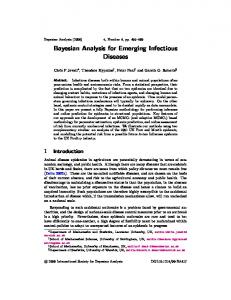
Originally the data set consisted of 76,800 cells corresponding to a grid of 240 by 320. With a large “population” such as this, calculation of the likelihood can become computationally prohibitive. Therefore the data set was aggregated to reduce the number of cells. Each set of 5 by 5 cells were aggregated to obtain a 48 by 64 grid composed of 3072 aggregated cells. The state of the aggregated cell was defined via a threshold classifying the aggregated cell as state B (burning) if 5 or more of the 25 smaller cells were burning; state O (burnt out) if there were more burnt out than untouched, and fewer than 5 burning smaller cells; and C (cold) if there were more untouched than burnt out, and fewer than 5 burning cells. Finally, the data set was cleaned in order to ensure that the state of a cell could take on the following transitions only: C → B, B → O, or C → O. It would be possible to relax these assumptions (e.g. allow C → B → C) but this is not considered here. The snap shots from the aggregated fire spread are shown in Figure 1.
620
Combustion Modelling Using ILMs
Various aggregation schemes were tested, and the models fitted produced qualitatively similar results (e.g. combustion simulations). For example, under an alternative aggregation scheme the original cell count of 76,800 cells was reduced to 19,200 aggregated cells. The state of these cells (corresponding to a coarser aggregation grid of 120 by 160) was found using a similar threshold technique as described above. The analysis of the data under this alternative aggregation scheme led to very similar conclusions as under the scheme used throughout the rest of this paper; e.g. rankings of the deviance information criterion (DIC) (Spiegelhalter et al. 2002) under each model – see Section 4 – were identical under both aggregation schemes.
3
Modelling
In this section, eight different models are considered for fitting the combustion pattern data described in Section 2.1. As discussed previously, the combustion pattern was digitalized at 14 time points through the course of the fire. These observations points were separated by time intervals (measured in seconds): 1.64, 0.40, 0.47, 0.46, 2.00, 1.00, 0.54, 0.53, 0.47, 0.46, 0.54, 0.46, 0.54, and 0.53. Some of the models described here do not account for differences between these time intervals. In effect, this is equivalent to assuming that the time intervals are identical and – in the context of the notation to be introduced in Section 3.3 – equal to ∆(t) = 1, (i.e. τt+1 − τt = 1).
3.1
Basic Geometric Kernel Model
The distance kernel for this first model is based on the simple power law, κ(dij ) = dij −β . With the equal time intervals assumption, the probability that cold cell i will become ignited at time t is given by
P (i, t) = 1 − exp −α
X
, d−β ij
α > 0, β > 0
(4)
j∈B(t)
where α is the combustibility constant and β is the power-law or decay parameter. An increase (decrease) in α represents an increase (decrease) in the overall strength of the fire, whereas a decrease (increase) in β represents a fire which spreads more quickly (slowly) through space.
3.2
Basic Exponential Kernel Model
In the second model the distance kernel is changed to κ(dij ) = exp{−βdij } where once again, β is the shape parameter of the kernel. Once again, assuming the time intervals between two consecutive observed times are equal, the probability that cold cell j ignites
I. Vrbik et al.
621
within the time interval [t, t + 1) is given by
P (i, t) = 1 − exp −α
X
exp{−βdij } ,
α > 0, β > 0
(5)
j∈B(t)
where α and β are parameters to be estimated. Since the exponential kernel was found to outperform the geometric kernel in terms of DIC, in the remainder of this section, models incorporating the geometric kernel are not presented.
3.3
Interval-Dependent Exponential Kernel Model
In the above models no attempt is made to account for the fact that the time intervals in between which the data were collected are not equal. The model here incorporates the fact that the data analyzed here was not collected at regular time points. The probability that cell i ignites within time interval [τt , τt+1 ) is now defined by X exp{−βdij } (6) P (i, t) = 1 − exp −α ∆(t) j∈B(t)
where ∆(t) = τt+1 −τt . The ∆(t) acts as a weight, making the probability of combustion, P (i, t), larger for longer time periods. This model with the geometric kernel replacing the exponential kernel was also fitted (results not shown).
3.4
Change Point, Exponential Kernel Model
A visual inspection of the data suggests that the combustion rate slows down at some point in time. Therefore, a model is considered that allows α and β to change at some time point k. The probability that cell i ignites within time interval [τt , τt+1 ) is now defined by i h 1 − exp −α1 ∆(t) P if t < k j∈B(t) exp{−β1 dij } h i P (i, t) = (7) P 1 − exp −α2 ∆(t) if t ≥ k j∈B(t) exp{−β2 dij } where α1 , α2 , β1 and β2 are all parameters to be estimated. This model is fitted for k = 2, ..., 13. Once again, the equivalent model with the geometric kernel replacing the exponential kernel was fitted but the geometric kernel did not perform as well as the exponential kernel according to their DIC values (results not shown).
3.5
Nearest Neighbour Kernel Model
An intuitive alternative to the exponential kernel is the nearest neighbour (NN) kernel. This leads to a model in which the probability that cell i ignites in the interval [τt , τt+1 )
622
Combustion Modelling Using ILMs
is now defined as X P (i, t) = 1 − exp −α I [dij < r]
(8)
j∈B(t)
where α is the only parameter to be estimated. The neighbourhood radius, r, in which we classify a nearest neighbour is set to 4 units since combustion patterns in the original data never exceed a jump of more than 4 cell units away from a burning cell. The distance kernel is now an indicator function where ½ I[dij < 4] =
3.6
1 if dij < 4 0 if dij ≥ 4.
Nearest Neighbour Exponential hybrid I Model
Here a hybrid of the nearest neighbour model and exponential kernels is considered. Including the exponential kernel allows the probability of combustion to vary depending on the distance within the defined neighbourhood. Here the probability of cell i igniting at interval [τt , τt+1 ) is
P (i, t) = 1 − exp −α
X
I[dij < r] exp{−βdij }
(9)
j∈B(t)
where once again r = 4 is used and α and β are parameters to be estimated.
3.7
Nearest Neighbour Exponential hybrid II Model
A potential problem with the previous model is that the probability of combustion for “long distance” cells (i.e. cells farther away than 4 units) is set to be 0. Here, a model is considered that still allows for long distance combustion with the added component of the nearest neighbour indicator function to add an extra weight to the neighbouring cells. The probability of individual i igniting within interval [τt , τt+1 ) is now P (i, t) = 1 − exp −α
X
I[dij < r] + exp{−βdij }
(10)
j∈B(t)
where I[dij < r] is the indicator function described in the previous section; α and β are parameters to be estimated; and the nearest neighbour radius r is set to 4.
623
β
6000 4000 0
0
2000
5000
α
10000
8000
15000
10000 12000
20000
I. Vrbik et al.
1.5
2.0
2.5
3.0
1.05
iteration
1.10
1.15
1.20
1.25
iteration
β 1.5
1.05
1.10
2.0
1.15
α
2.5
1.20
1.25
3.0
(a) Marginal posterior distributions
0e+00
2e+04
4e+04
6e+04
8e+04
1e+05
0e+00
iteration
2e+04
4e+04
6e+04
8e+04
1e+05
iteration
(b) Trace plots after convergence
Figure 2: Marginal posterior distributions and trace plots under the basic exponential distance kernel model.
3.8
Log-Normal Beta
Finally, a model in which β can vary over time in a flexible or natural manner is considered. This flexible model now defines βt = f (t) where f (t) is a log-normal curve. A non-negative truncated normal prior with variance 5000 is put on the parameters of the lognormal curve; µ, σ and A. The probability that cell i ignites within time interval [τt , τt+1 ) is now defined by P (i, t) = 1 − exp −α
X
exp{−βt dij }
j∈B(t) 2
}; now θ = (α, A, µ, σ) are to be estimated. where βt = A exp{ −(logσt−µ) 2
(11)
20
40
60
40 x
60
40 y
20 0
y
40
60
0
20
40
60
40
60
40
60
y
40
x
40
0
y
20
0
20
40
60
0
20 x
y
40
x
40
0
y
20
40 x
0
0 0
20
0 0
40 y
0
x
20
40
60
60
0 0
x
40 x
40
40 y
40 y
60
20
20
20 x
0 40
0 0
0 0
20
60
20
40 y
20
20 x
y
40
20
40 20 x
0 0
20
y
0
20
60
20
40 x
20
20
20
0
0
y
20 0
20 0
y
40
Combustion Modelling Using ILMs
40
624
0
20
40
60
x
0
20
40
60
x
Figure 3: Typical simulation for the exponential kernel model with the marginal posterior means substituted in for parameters.
3.9
Fitting the Models and the Data
The models are fitted in a Bayesian framework which combines the likelihood with the prior distribution to obtain the posterior distribution for θ. Since we want to restrict the parameter space to that of R+ , with little prior knowledge, we assume the prior distribution for all parameters follow a normal distribution with mean 0 and variance 5000 and truncate the normal distribution to include only non-negative values. Random walk Metropolis-Hastings MCMC (e.g. Gamerman and Lopes 2006) is used in order to obtain a sequence of random samples from the posterior distribution. The random-walk proposal used for all parameters is the uniform, with range tuned to produce acceptably efficient mixing. For all models, the random-walk Metropolis Hastings MCMC algorithm was run for 100,000 iterations including a burn-in period of 2000 iterations. Convergence was verified visually. For illustration, see Figure 2(a) for the marginal posterior distributions, and Figure 2(b) for the trace plots, of the parameters of the exponential kernel model after convergence, as well as a typical simulation of that model under the posterior means of the parameters shown in Figure 3.
I. Vrbik et al. Table 1: Parameter posterior mean values. Model Parameter Posterior Mean Geometric Kernel Model α 1.937 β 3.665 Exponential Kernel Model α 2.079 β 1.149 Interval-dependent Model α 4.050 β 1.183 † Change Point Model k = 5 α1 1.369 α2 5.570 β1 0.923 β2 1.274 NN Kernel α 0.202 NN Exponential hybrid I α 4.327 β 1.155 NN Exponential hybrid II α 0.092 β 0.628 Log-Normal Beta α 2.103 A 2.707 µ 60.621 σ 70.415 †
625
95% PI (1.717, 2.177) (3.568, 3.759) (1.725, 2.471) (1.091, 1.208) (3.343, 4.876) (1.123, 1.244) (0.900, 1.965) (4.480, 6.767) (0.826, 1.019) (1.201, 1.344) (0.188, 0.216) (3.184, 5.698) (1.0344, 1.273) (0.085, 0.099) (0.594, 0.662) (1.716, 2.519) (1.187, 5.773) (9.186, 142.341) (25.447, 143.493)
The results for other change points (k = 2, ..13) can be found in Figure 4.
4
Results
The mean posterior parameter values and their 95% percentile intervals are given in Table 1 and Figure 4. Models were compared in three ways. First, a comparison between plots of simulated data from each model under the posterior means, and the observed data, was made. Second, models were compared using the deviance information criterion (DIC) (Spiegelhalter et al. 2002). The DIC values obtained for each model, along with the ranks (1 being the model with the lowest DIC), are given in Table 2. The third method of comparison consisted of considering the one-step-ahead posterior predictive distribution of the number of burning cells over the course of the experiment for each model. This is discussed in Section 4.8. First, we consider comparing the models via direct simulation and the DIC.
4.1
Exponential and Geometric Kernel Model
When the basic distance kernel models are compared, the exponential model performs better in terms of DIC. In Figure 5(a) the probability of susceptible cell i catching fire from single burning cell j is plotted against the Euclidean distance dij (the kernels
Combustion Modelling Using ILMs
15
α2
0
5
50
10
100
α1
150
20
200
626
2
4
6
8
10
12
2
4
6
8
10
12
8
10
12
k
1.3
β2
1.0
1.0
1.1
1.2
1.5
β1
2.0
1.4
1.5
2.5
1.6
k
2
4
6
8
k
10
12
2
4
6
k
Figure 4: Posterior mean estimates and 95% credible intervals of the Change Point, Exponential Kernel Model parameters for different values of the change-point parameter, k = 1, ...12.
themselves are shown in Figure 5(b)). Naturally it is expected that the farther away burning cell j is from i the lower the probability of combustion. Both models follow this assumption. However, it can be seen that the fitted exponential model allows for probabilities less than 1 when dij = 1, whereas the fitted geometric model produces a probability plot with a plateau at 1 which then rapidly drops to 0. This results in the exponential kernel model having a degree of randomness at small distances which the geometric kernel model does not. It may be this discrepancy that results in the geometric model having a weaker fit. The heavy tails of the geometric model also may contribute to its lack of fit since having non-zero probabilities for long distances may not be realistic for this combustion data.
I. Vrbik et al. Table 2: Deviance Information Criterion (DIC). Model Submodel DIC Geometric Kernel Model 3610.202 Exponential Kernel Model 3456.496 Interval-dependent Model 3390.024 Parameter Change Point k=1 3360.836 k=2 3356.067 k=3 3360.338 k=4 3347.073 k=5 3343.684 k=6 3355.261 k=7 3374.983 k=8 3385.637 k=9 3385.736 k = 10 3385.804 k = 11 3379.686 k = 12 3357.953 Nearest Neighbour Kernel 7363.945 Nearest Neighbour Exponential hybrid I 7133.889 Nearest Neighbour Exponential hybrid II 3718.784 Log-Normal Beta 3329.293
627
Rank 5 4 3
2
8 7 6 1
The plots of a typical simulation under the posterior means for the exponential and geometric kernel models are shown in Figures 3 and Figure 6, respectively. Comparing these to the aggregated snap shots (Figure 1) the exponential model produces a fire spread shape with smooth edges and non-circular features that is similar to that of the original data. The geometric model on the other hand produces spread patterns with many jumps and jagged edges that are not representative of the original data. For both models the rate of the fire spread is too fast, with nearly all the cells in the burnt out state by the last time interval.
4.2
Interval-dependent Model
Compared to the equal interval exponential kernel model, accounting for the varying time intervals improves the model fit with a reduction of 66.472 in the DIC (3456.496 – 3390.024). This is no surprise, since the time intervals ranged from 0.40s to 2.00s and it would be expected that the fire would spread more in a longer interval than a shorter one.
Combustion Modelling Using ILMs
1.0 0.8
0.8
0.6
Exponential Geometric
0.0
0.2
0.2
0.4
0.4
κ(dij)
0.6
Exponential Geometric
0.0
Probability of i catching fire from j
1.0
628
0
1
2
3
4
5
6
7
0
1
2
dij
(a) Pit vs dij
3
4
5
6
7
dij
(b) κ(dij ) vs dij
Figure 5: (a) The probability of susceptible cell i catching fire from burning cell j; and (b) distance kernel κ(dij ); both plotted against dij for the exponential kernel (solid line) and the geometric kernel (dotted line) under the posterior means.
4.3
Change Point, Exponential Kernel Model
For the parameter change point model, all possible values of the change point k are considered. The model with k = 5 produces the lowest DIC of 3343.684. This model also appears to offer an improvement over the interval-dependent model with a DIC that was reduced by 46.340 (3390.024 – 3343.684). Although the inclusion of change points results in a model that slows the fire down for the second half of the fire, simulations under the posterior mean still produce a faster fire spread than seen in the original data (results not shown). The posterior mean estimates, and 95% credible intervals of the model parameters are are given in Figure 4. Another alternative is to treat k as a parameter to be estimated. Using this technique the same method was conducted on this 5 parameter model and the marginal posterior mean for k was found to be 6.511438.
4.4
Nearest Neighbour (NN) Kernel Model
The nearest neighbour model, although intuitively sensible for fire spread, did poorly in terms of the DIC. The NN kernel model results in a two-fold increase in DIC value compared to that of the change point exponential kernel model. As can be seen in Figure 7, the NN model typically produces a circular pattern that fails to mimic the observed data’s elliptical-like pattern.
20
40
60
40
60
40 y
20 0
y
40
60
0
20
40
60
40
60
40
60
y
40
x
40
0
y
20
0
20
40
60
0
20 x
y
40
x
40
0
y
20
40 x
0
0 0
x
20
0 0
40 y
0
x
20
40
60
60
0 0
x
40
40
40 y
40 y
60
20
20
20 x
0 40
0 0
0 0
20
60
20
40 y
20
20 x
y
40
20
40 20 x
0 0
20
y
0
20
60
20
40 x
20
20
20
0
0
y
20 0
20 0
y
40
629
40
I. Vrbik et al.
0
20
x
40
60
0
20
x
40
60
x
60
20
40
60
40 x
60
40 y
20 0
y
40
60
0
20
40
60
40
60
40
60
y
40
x
40 y
20
0
20
40
60
0
20 x
y
40
x
40
0
y
20
40 x
0 0
20
0 0
40 y
0 60
0
x
20
40 20
40 x
60
0 0
x
0
20
40
40 y
40 y
40 x
0
20 x
0 20
0 0
20
60
20
40 y
20 0 0
y
40 x
0
20
20
40 y
0 0
20
60
20
40 x
20
20
20
0
20
40 y
20 0
20 0
y
40
Figure 6: Typical simulation for the geometric kernel model with the marginal posterior means substituted in for parameters.
0
20
40 x
60
0
20
40
60
x
Figure 7: Simulation of the nearest neighbour model with the marginal posterior means substituted in for parameters.
630
4.5
Combustion Modelling Using ILMs
NN Exponential hybrid I Model
The first hybrid model that used the exponential kernel in conjunction with the nearest neighbour indicator function offers a slight improvement over the original nearest neighbour model. The DIC for this model (7133.889) is lower than that of the NN kernel model (7363.945). However, this model is still poor in terms of DIC value compared to the other non-NN models considered.
4.6
NN Exponential hybrid II Model
The nearest neighbour exponential hybrid II model produces a much smaller DIC value (3718.783) comparing to the simple NN model (7363.945). This model allows for long distance incidence of combustion while providing an added weight to those burning cells being the nearest neighbour of cell i. However, the DIC values suggest that the second hybrid model does not perform better than the non-NN models.
4.7
Log-Normal Beta Model
The log-normal beta model with four parameters yields the smallest DIC of 3329.293. Separate probability curves for each time point t = 1, ...14 do not appear to differ greatly for different values of t. However, this flexibility seems to offer a better fit over other models. In addition, this model generates the fire combustion pattern that best matches the pattern of original data with a much lower combustion rate compared to other models (although the combustion rate is still not as low as observed in the original data). The simulated pattern based on the log-normal beta model is shown in Figure 8.
4.8
Posterior Predictive Checks
Further model comparisons can be made via the one-step-ahead posterior predictive distribution of the number of burning cells over the course of the experiment for each model. The one-step-ahead posterior predictive distribution of the number of burning cells at time B is found in the following way. First, model parameters are sampled from the posterior distribution estimated via MCMC for a given model. Second, the combustion pattern at time B + 1, conditional upon the data up to time B is simulated from the given model using the posterior-sampled parameter values. Third, the number of burning cells at time B + 1 is recorded. Note that cells observed to go from the burning to burnt out states from times B to B + 1 are assumed to burn out in the one-step simulation. This three-step procedure is repeated 100 times for each of B = 2, . . . , 13. The resulting one-step-ahead posterior predictive distributions of the number of burning cells over time, for six of the eight models fitted, are shown in Figure 9. These distributions can be compared with the observed data, superimposed on the plots in black. Note that, one-step-ahead posterior predictive plots of two of the models fitted are not shown for reasons of brevity. First, the plot for the geometric kernel model is very similar to that
20
40
60
40 x
60
40 y
20 0
y
40
60
0
20
40
60
40
60
40
60
y
40
x
40
0
y
20
0
20
40
60
0
20 x
y
40
x
0
0 20
40 x
40 y
40 y
0 0
20
x
20
40
60
0
0 0
x
40
60
0 0
x
40
40 y
40 y
60
20
20
20 x
0 40
0 0
0 0
20
60
20
40 y
20
20 x
y
40
20
40 20 x
0 0
20
y
0
20
60
20
40 x
20
20
20
0
0
y
20 0
20 0
y
40
631
40
I. Vrbik et al.
0
20
40 x
60
0
20
40
60
x
Figure 8: Simulation of the log-normal beta model with the marginal posterior means substituted in for parameters.
of the exponential kernel model. Secondly, the plot for the change point exponential kernel model is very similar to that of the interval-dependent exponential model. In both cases, only the plots for the latter of the two models are included. For the most part the posterior predictive plots follow the general trend of the burning cell count curve. However, as we can see from Figure 9 the non-nearest-neighbourbased models all tend to overestimate the number of burning cells. It also appears from the posterior predictive plots that there is little to differentiate between those models (including the two models for which plots are not shown – see above). We see from the plots for the NN kernel model and the NN exponential hybrid II model that both of these models tend to underestimate the number of burning cells for the second half of the experiment. Of the models tested, the posterior predictive plot for the NN exponential hybrid I model seems to suggest that this model fits the data best. However, even this fit could only probably be described as moderately good, and is not a vast improvement over, say, the log-normal beta model’s.
5
Conclusions
In this paper a variety of ILMs were considered as tools for modelling the spatio-temporal dynamics of fire spread for a particular data set under controlled conditions. To some extent, at least some of the fitted models were able to produce simulated data with a
200 150 0
50
100
Number of Burning Cells
200 150 100 0
50
Number of Burning Cells
250
Combustion Modelling Using ILMs
250
632
2
4
6
8
10
12
2
4
Time Interval
10
12
250 200 150 0
50
100
Number of Burning Cells
200 150 100 0
50
Number of Burning Cells
8
(b) Interval-dependent Exponential Model
250
(a) Exponential Kernel Model
2
4
6
8
10
12
2
4
Time Interval
6
8
10
12
Time Interval
200 150 100 50 0
0
50
100
150
200
Number of Burning Cells
250
(d) NN exponential hybrid I model
250
(c) NN Kernel Model
Number of Burning Cells
6
Time Interval
2
4
6
8
10
12
Time Interval
(e) NN exponential hybrid II model
2
4
6
8
10
12
Time Interval
(f) Log-normal beta model
Figure 9: One-step-ahead posterior predictive distribution of the number of burning cells for various models; black curves show the observed data and blue curves are posterior predictive realizations.
I. Vrbik et al.
633
combustion pattern similar in terms of shape and variability to that of the original fire spread data. However, in general, the combustion patterns generated by these models tended to burn at a faster rate than the original observed combustion pattern. It was observed that models with an exponential distance kernel performed better in terms of minimizing DIC than models with a geometric distance kernel. The preference of an exponential kernel is consistent with the wave-like progression of the fire observed in the data; the geometric kernel, having heavier tails than the exponential kernel, tends to result in more long distance spread. Models with purely nearest neighbour based kernels performed very poorly in terms of DIC. It was also observed that models which were, in some respects, heterogeneous over time, outperformed models which did not allow this heterogeneity. For example, the time-varying model outperformed the simpler, and otherwise equivalent, exponential kernel model; and the model that performed best in terms of DIC was the log-normal beta model, which allows the distance kernel to vary over time. There are a variety of other models that could be examined, and, indeed, many others were fitted but have not been included in this paper since they did not perform well (e.g. a model in which the β parameters follow an exponential curve, rather than a log-normal shaped curve). A comparison of the models using the one-step-ahead posterior predictive distribution of the number of burning cells, as well as simple simulation from the posterior means, seems to suggest that most of the models fitted tended to produce simulated combustion patterns that are more vigorous than that observed in the data. The three nearest neighbour based models were tested in the hope that they would produce less vigorous fires. It would appear that in this they were successful. In fact, in the case of the nearest neighbour kernel model, and nearest neighbour exponential hybrid II model, underestimation of the severity of the fire spread occurred. It should be noted that the model that seems to do best in terms of posterior predictive performance, the nearest neighbour exponential hybrid I model, had a much higher DIC than all of the non-nearest neighbour based models. It would appear that although this model seems to perform well in terms of its global behaviour, at the local level prediction is quite poor, and this is borne out by a lower log-likelihood. There are a number of issues that could be explored further. For example, in the likelihood, we assume that the newly burning cells are igniting independently of each other, conditional on the present configuration of burning cells. As fires tend to propagate as a wave, this assumption may not be very realistic for a fire. Relaxing this assumption may be desirable, although it would greatly increase the complexity of the likelihood function and probably introduce new computational difficulties to overcome. In this paper, we only consider the transition path C → B and B → O (and in some cases C → O might be recorded in the data, although this transition is not modelled as such, but merely recorded). However it is possible that a burning cell could become extinguished and therefore returns to the cold state C, before maybe reigniting later. Further, the likelihood of such a transition path for a cell would be expected to increase the larger the cells are. However, such transition paths are not considered among the proposed models. It would be interesting to investigate models that incorporate this
634
Combustion Modelling Using ILMs
possibility as it is a plausible occurrence in nature. Another thing that would be worthy of examination might be the rescaling of the models once the time intervals have been altered. The data was collected at 14 different time points over the life of the fire and it would be interesting, say, to investigate what would happen if the data was collected more often. This is especially important because it is being assumed in the interval-dependent models that a simple multiplicative rescaling of the α parameter is an adequate adjustment. The validity of the assumption should be tested in further work. In this paper, the burning state of each cell was ascertained initially by thresholding the RBG values in R, and then correcting the errors by eye to give us our observed data. Of course, a more satisfactory method of dealing with the above possible errors would be the use of random effects representing measurement error, incorporated into the analysis via data-augmented MCMC. This augmenting set of parameters would essentially represent the difference between the true and observed times at which the transitions from C → B and B → O occur. However, this augmentation would greatly increase the computational burden involved in the analysis. To facilitate practicable computation times, the observed data in our study was aggregated. The aggregation method used was very simple, and much more complicated methods for dealing with high dimensional spatial/spatio-temporal data could be considered. Three such examples in different settings are given by Higdon (1998), Calder (2008) and Cressie and Johannesson (2008). Cressie and Johannesson (2008) aim to approximate the variance-covariance matrix of fine gridded data by a sample of much more coarsely gridded data via a method based on yielding the best estimators of the covariance function parameter using the Frobenius norm. Higdon (1998) and Calder (2008) focus on a process convolution approach to modelling the variance-covariance matrix of spatio-temporal data to avoid a prohibitively high computational burden. The methods employed by these authors are designed for continuous responses such as the total column ozone (TCO) measures (Cressie and Johannesson, 2008); the ocean temperature (Higdon, 1998); and the concentration of the particulate matter (Calder, 2008). However, in our study, the response is categorical. Extension of one of the above, or similar, aggregation methods to our problem would, therefore, be non-trivial. Another issue of interest could be a comparison between empirically-led, ILM-based fire spread models, and those are derived from more fundamental physical and/or theoretical assumptions, such as FARSITE and Prometheus. For example, both of these models follow the aforementioned Huygens principle in which waves propagate from points on the outer edge to determine the position of the fire front at specific times. However, there is no reason why an ILM-based fire spread model should follow this principle. At best, an ILM, which is of course a stochastic model, could be constructed to follow the Huygens principle in its mean behaviour. However, in the models tested in this paper, the fact that the fire spread can occur in all directions from the wave front means that the Huygens principle is not followed. Finally, it would be very interesting to apply ILMs to forest fire data. In doing so, the susceptibility and transmissibility functions of the general form of the ILM could allow
I. Vrbik et al.
635
topographical covariates, and information on things such as forest type and density, etc., to be included as risk factors. Such models could also be extended to include meteorological data, either in a static sense where the distance kernel could allow for a prevailing wind direction, or a dynamic sense in which the kernel could vary over time, informed by updated meteorological information. It would seem, at least intuitively, that the use of time-varying parameters would likely provide a better strategy for forest fire modelling than non-time-varying parameters, as it would be expected that the rate of fire growth would change over time with varying conditions.
References Beer, T. and Enting, I. G. (1990). “Fire spread and percolation modelling.” Mathematical Computer Modelling, 13: 77 – 96. 616 Berjak, S. G. and Hearne, J. W. (2002). “An improved cellular automaton model for simulating fire in a spatially heterogeneous Savanna system.” Ecological Modelling, 148: 133 – 151. 615, 616 Besag, J. (1972). “Nearest-Neighbour Systems and the Auto-Logistic Model for Binary Data.” Journal of the Royal Statistical Society, Series B, 34: 75 – 83. 619 Byram, G. M. (1959). Forest Fire: Control and Use, chapter Combustion of forest fuels, 65 – 89. New York: McGraw Hill. Ed: K. P. Davis. 616 Calder, C. A. (2008). “A dynamic process convolution approach to modeling ambient particulate matter concentrations.” Environmetrics, 19: 39 – 48. 634 Caragea, P. C. and Kaiser, M. S. (2009). “Autologistic Models With Interpretable Parameters.” Journal of Agricultural, Biological, and Environmental Statistics, 14: 281 – 300. 619 Cressie, N. and Johannesson, G. (2008). “Fixed rank kriging for very large spatial data sets.” Journal of the Royal Statistical Society, Series B, 70: 209 – 226. 634 Deardon, R., Brooks, S., Grenfell, B., Keeling, M., Tildesley, M., Savill, N., Shaw, D., and Woolhouse, M. (2010). “Inference for individual-level models of infectious diseases in large populations.” Statistica Sinica, 20: 239–261. 616 Finny, M. (1998). “FARSITE: Fire area simulator–Model development and evaluation.” United States Department of Agriculture Forest Service Research Paper RMRS-RP-4. 615 Gamerman, D. and Lopes, H. (2006). Markov chain Monte Carlo: stochastic simulation for Bayesian inference. Chapman & Hall/CRC Texts in Statistical Science, 2nd edition. 624 Garcia, T., Braun, J., Bryce, R., and Tymstra, C. (2008). “Smoothing and bootstrapping the PROMETHEUS fire growth model.” Environmetrics, 19: 836–848.
636
Combustion Modelling Using ILMs
Gelman, A., Carlin, J. B., Stern, H. S., and Rubin, D. B. (2004). Bayesian Data Analysis. Chapman & Hall, 2nd edition. Gibson, G. J. and Austin, E. J. (1996). “Fitting and testing spatio-temporal stochastic models with application in plant epidemiology.” Plant Pathology, 45: 172–184. Higdon, D. (1998). “A process-convolution approach to modelling temperatures in the North Atlantic Ocean.” Environmental and Ecological Statistics, 5: 173 – 190. 634 McArthur, A. G. (1966). “Weather and grassland fire behaviour.” Leaflet 100, Australian Forestry and Timber Bureau. Neal, P. J. and Roberts, G. O. (2004). “Statistical inference and model selection for the 1861 Hagelloch measles epidemic.” Biostatistics, 5: 249–261. Noble, I. R., Bary, G. A. V., and Gill, A. M. (1980). “McArthur’s fire-danger meters expressed as equations.” Australian Journal of Ecology, 5: 201 – 203. Ntaimo, L., Zeigler, B. P., Vasconcelos, M. J., and Khargharia, B. (2004). “Forest fire spread and suppression in DEVS.” Simulation, 80: 479 – 500. 616 Perry, G. L. W. (1998). “Current approaches to modelling the spread of wildland fire: a review.” Progress in Physical Geography, 22: 222 – 245. 616 Podur, J., Martell, D. L., , and Knight, K. (2002). “Statistical quality control analysis of forest fire activity in Canada.” Canadian Journal of Forest Research, 32: 195–205. R Development Core Team (2009). R: A Language and Environment for Statistical Computing. R Foundation for Statistical Computing. 617 Rothermel, R. C. (1972). “A mathematical model for predicting fire spread in wildland fuels.” Research Paper INT - 115, USDA Forest Service. 616 Spiegelhalter, D., Best, N., Carlin, B., and van der Linde, A. (2002). “Bayesian measures of model complexity and fit.” Journal of the Royal Statistical Society, Series B, 64: 583–639. 620, 625 Tymstra, C., Bryce, R. W., Wotton, B. M., and Armitage, O. B. (2010). “Development and structure of Prometheus: the Canadian wildland fire growth simulation model.” National Resources Canada, Canadian Forest Services Information Report NOR-X417. 615, 616 Waltman, P. and Hoppensteadt, F. (1970). “A Problem in the Theory of Epidemics I.” Mathematical Biosciences, 9: 71 – 91. 617 — (1971). “A Problem in the Theory of Epidemics II.” Mathematical Biosciences, 12: 133 – 145. 617 Zheng, Y. and Zhu, J. (2008). “Markov chain Monte Carlo for a Spatial-Temporal Autologistic Regression Model.” Journal of Computational and Graphical Statistics, 17: 123 – 137. 619
I. Vrbik et al.
637
Acknowledgements This work was funded in part by the Natural Sciences and Engineering Research Council (NSERC) of Canada Discovery Grants Program and GEOIDE.
638
Combustion Modelling Using ILMs