Application to the Apache Web Server. Yixin Diao. 1 .... in the design and analysis of feedback control to enforce policies in the presence of such interactions.
Using MIMO Feedback Control to Enforce Policies for Interrelated Metrics With Application to the Apache Web Server Yixin Diao1 , Neha Gandhi2 , Joseph L. Hellerstein3 , Sujay Parekh4 , and Dawn M. Tilbury5 IBM T. J. Watson Research Center1−5 {diao, hellers, sujay}@us.ibm.com Department of Mechanical Engineering, University of Michigan2,5 {gandhin, tilbury}@umich.edu Abstract Policy-based management provides a means for IT systems to operate according to business needs. Unfortunately, there is often an “impedance mismatch” between the policies administrators want and the controls they are given. Consider the Apache web server. Administrators want to control CPU and memory utilizations, but this must be done indirectly by manipulating tuning parameters such as MaxClients and KeepAlive. There has been much interest in using feedback control to bridge the impedance mismatch. However, these efforts have focused on a single metric that is manipulated by a single control and hence have not considered interactions between controls such as those that are common in computing systems. This paper shows how multiple-input, multiple-output (MIMO) control theory can be used to enforce policies for interrelated metrics. MIMO is used both to model the target system, Apache in our case, and to design feedback controllers. The MIMO model captures the interactions between KA and MC, and can be used to identify infeasible metric policies. In addition, MIMO control techniques can provide considerable benefit in handling trade-offs between speed of metric convergence and sensitivity to random fluctuations while enforcing the desired policies. Keywords Web Server, Resource Management, Policy-based management, Control Theory, MIMO Control
1 Introduction The wide-spread exploitation of information technology (IT) has motivated the need for policy-based management of IT resources. For example, a business may have policies that limit the memory and CPU consumed by web servers. These policies originate from several business needs, including: (a) providing sufficient capacity to co-located applications (e.g., file server, database server); (b) avoiding thrashing and failures as a result of overutilization; and (c) ensuring that there is sufficient capacity remaining to handle workload surges and/or server failures. Herein, we describe a control-theory based approach to enforcing policies for interrelated metrics, and we apply this approach to the Apache [1] web server.
MEM
CPU
Frequently, there is an “impedance mismatch” between the policies administrators want and the controls they are given. For example, in an Apache web server, administrators want to control the CPU and memory utilizations (hereafter denoted by CPU and MEM) associated with the Apache application, but there is no way to do this directly. Rather, administrators must operate indirectly by adjusting various tuning parameters. The operations staff must conduct experiments to determine how desired utilizations can be achieved with the controls that are available. Two widely used parameters are MaxClients (MC), the maximum number of clients that can connect to an Apache server, and KeepAlive Timeout (KA), which determines how long an idle connection is maintained in HTTP 1.1. Light Workload (2 sess/sec)
1
1
0.5
0.5
0 1
0 1
0.5
0.5
0 0
50
100
150 200 Time(s)
Heavy Workload (20 sess/sec)
250
0 0
300
50
100
150 200 Time(s)
250
300
Figure 1: Effect of Static Settings with KA = 6 and MC = 450. Note that CPUincreases from 35% with the light workload to 50% with the heavy workload. Not surprisingly, it is time-consuming, error-prone, and skills intensive to manually adjust MC and KA to achieve desired settings of CPU and MEM. Even worse, this effort has to be repeated as the workload changes. This is illustrated in Figure 1, which shows how CPU and MEM are affected as the workload changes from light to heavy. (The precise definition of light and heavy are discussed later.) While MEM changes little, CPU increases from 35% in the light workload to 50% in the heavy workload. (
&38 0
$
G
P
(0
&38
�
�
( 0
(0
&R
Q
W U R
O O H
U
$ 0
.
$ &
S 6
D H
F K U Y
&38 H
H
U
0
(0
L Q
Figure 2: Block Diagram of Feedback System for Control of CPU and Memory Utilizations We propose using feedback control to bridge the gap between administrative goals and IT controls. The specifics are shown in Figure 2. We assume that there are policies for CPU and MEM, in terms of the desired values of these metrics, denoted by CPU* and MEM* respectively. The controller reads measured values1 of CPU and MEM, and computes the control error. The CPU control error is denoted by ECP U = CPU∗ −CPU. EM EM is defined analogously for MEM. The controller uses current and past values of 1 We use time-averaged values to reduce measurement overhead and also because the inherent variability of the metrics (CPU utilization in particular) makes instantaneous control impractical.
+
CPU*
ECPU C1
MEM* +
C2
SISO
KA MC
CPU MEM
SISO
- E MEM
(a) Model: SISO Controller: SISO
ECPU
+
CPU* MEM*
C
KA
CPU MIMO
MC
MEM
+
- E MEM
(b) Model: MIMO Controller: MIMO
Figure 3: Architectures for Feedback Control of Apache control error to adjust MC and KA with the goal of achieving the desired target utilization values (i.e., ECP U ≈ 0 ≈ EM EM ). Control theory provides sound and rigorous mathematical principles to analyze dynamical systems, and design controllers for them. While it is widely used in mechanical, aeronautical, and chemical engineering [2], there is concern with applying standard linear control techniques to computer systems, a domain in which non-linearities abound. Although there is a well-developed theory of non-linear control, it is much more difficult to apply, does not generalize across systems, and provides much less insight than linear control theory. Hence, we adopt a pragmatic perspective. Can we construct and analyze the properties of real-life closed-loop computer systems using linear control theory? Prior work in applying control theory to computing systems has focused on singleinput, single-output (SISO) techniques in which there is a single control and a single metric to regulate. Examples include flow and congestion control [3], [4], differentiated caching [5], multimedia streaming [6], differentiated web services [7] and control of an email server [8]. In some cases [7], [5], where the system is multiple-input, multipleoutput (MIMO), the approach taken is to decompose into multiple simpler, independent SISO control loops. However, in many cases, complex systems cannot be decomposed because of interactions between the controls. The main contribution of this paper is the use of the more general MIMO techniques in the design and analysis of feedback control to enforce policies in the presence of such interactions. The two approaches to controlling a MIMO system are shown in Figure 3. As seen in Figure 3(b), MIMO is used in two ways: (1) to model and predict the behavior of the Apache server and (2) to design the controller. We show that SISO models are not able to accurately model CPU because of the interaction between KA and MC; a MIMO model works better. Further, we show that having an accurate model of CPU and MEM is particularly useful for accurately determining the space of feasible policies for these metrics. In terms of control, it turns out that for our system using independent, simpler SISO controllers (Figure 3(a)) works surprisingly well inspite of the SISO modeling inaccuracies. This is due to the limited nature of the interactions between KA and MC. However, we show that MIMO techniques such as linear quadratic regulation (LQR) can provide considerable benefit in terms of balancing the trade-off between speed of convergence to the desired result and sensitivity to random fluctuations. We also note that in many of the aforementioned studies, the focus has been on using first principles models for which little empirical validation is done. By contrast, we proceed along the lines of the work in [8] in which empirical models are developed and
validated for an email server. Other research on improving web server performance is in the areas of admission control schemes [9], adaptive content delivery [10], caching [11] and other mechanisms [12]. In these, the focus has been on client-perceived metrics such as response time. To the best of our knowledge, ours is the first work that discusses the tuning of server parameters for goals related to administrative policies. The remainder of this paper is organized as follows. Section 2 provides background on the Apache architecture and our modifications for enabling feedback control. Section 3 details our approach to MIMO modeling and compares the results to the models obtained with a SISO model. Section 4 presents and evaluates several controller designs. Our conclusions are contained in Section 5.
2 Apache Architecture and Enabling Dynamic Control Apache v1.3 on Unix [1] is structured as a pool of worker processes monitored and controlled by a master process, as shown in Figure 4. The worker processes are responsible for handling the communications with the Web clients, including the work required to generate the responses. A worker process handles at most one connection at a time, and it continues to handle only that connection until the connection is terminated. Thus, the worker is idle between consecutive requests from its connected client. The MC parameter limits the size of this worker pool, thereby imposing a limitation on the processing capacity of the server. A higher MC value allows Apache to process more client requests. But if MC is too large, there is excessive resource consumption that degrades performance for all clients. U HS
7
O \
1HZ� 8
V HU V &
7
L P
HR
X
O R
%
V H�
X
V
W �
8 \ 7
U HT
X
HV
6 7
.,//
R
Q
HR
&
�
1HZ�F
L P
Q :
7 /
&
R
U N
HU V 6
3
$
:
0
D
V
W HU &
R
Q
W U R
V K
O R
X
W
H
HU L Q
, N
W
&
HU Y HU �6
W D
U D
V
Q
V L W L R
R
Q
Q
HF
G
O H
W
Q
W H� V
O O HU
1
3
T
L V W HQ X
HX
H
MaxClients KeepAlive 6
F
R
U HE
$
S
R
D
D
U G
F
K
H
Figure 4: Apache architecture and session flow Figure 4 contains a state transition diagram for worker processes. In the “Idle” state, a worker is waiting for a client connection, at which point it enters the “User Think” state and waits for an HTTP request. The worker is in “Busy” for processing the request and sending a reply. The time between sending an HTTP reply and the receipt of the next request (for HTTP/1.1 persistent connections [13]) is spent in the “User Think” state and is known as user think time. The Apache KA tuning parameter controls the maximum time a worker can remain in the “User Think” state before its client TCP connection is closed, thus allowing the worker to handle other clients. If KA is too large, CPU and memory are underutilized since clients with requests to process cannot
connect to the server. Reducing the timeout value means that workers spend less time in the “User Think” state, and CPU increases. If the timeout is too small, however, the TCP connection terminates prematurely and reduces the benefits of having persistent connections. In order to dynamically control Apache, we needed to (1) have programmatic access to performance metrics and (2) be able to set the tuning parameters on-line. To facilitate these capabilities, we have implemented a control module that provides a GET/SET interface over a special TCP port. Metrics are stored in the Apache scoreboard (a shared memory area common to all the Apache processes) and updated asynchronously. For control, we converted the MC and KA static configuration parameters into variables accessed through the scoreboard, and changes to them are picked up asynchronously by the affected components at some convenient time in their processing. Another major change to Apache for dynamic control concerns the effect of MC. The unmodified Apache incorporates a heuristic to dynamically change the server pool size based on the two parameters MinSpareServers and MaxSpareServers. Since we would like our controller to replace this heuristic, we modified the effect of MC so that it directly controls the size of the worker pool. The master process creates or kills worker processes to ensure that the total pool size matches the MC value specified by the controller. Note that although we have slightly changed the semantics of MC, this does not affect Web Administrators since they do not have to set MC anymore.
3 Modeling Apache This section describes our approach to modeling Apache, which is based on statistical (“black box”) models to quantify the relationship between the tuning parameters (KA and MC) and metrics (CPU and MEM). We first describe the experimental environment used to obtain the data from which the models are constructed. Then we describe our models, and briefly evaluate them. In Section 3.4, we show how the models can be used to determine feasible policies (e.g., realizable combinations of CPU and MEM) and to predict the dynamic behavior of the system.
3.1 Experimental environment Our testbed consists of one server running Apache connected through a 100Mbps LAN to one or more clients running a synthetic workload generator. The server is a Pentium III 800 MHz with 256MB RAM, running Linux. Each client machine runs a synthetic workload generator described below that simulates the activity of many clients. , Q
W HU �V HV V LR
Q
7LPH 7K
LQ
N
� 7LPH
%
X
U V W
Figure 5: Depiction of Workload Model. Two sessions are displayed as indicated by the solid and dashed arrows. The long arrows denote clicks, and the short arrows indicate the objects in a burst. Our workload generator uses the publicly-available httperf [14] at its core to generate HTTP/1.1 requests and manage user sessions. We have written wrapper scripts
to emulate a stochastic user behavior as described by the WAGON model of Liu et al [15]. As shown in Figure 5, WAGON structures the workload into multiple sessions (which represent a series of user interactions) during which there are multiple clicks (end-user requests), each of which generates a burst of HTTP requests (which represents web pages with multiple objects). Thus, the workload parameters are: session arrival rate, number of clicks in a session, burst size (number of objects in a burst), and think time (distribution of time between clicks). Table 1 summarizes the parameters we used, which is based on the data reported in [15]. The file access distributions we use are from the Webstone 2.5 reference benchmark [16]. Based on the findings in [15], our session arrivals are Poisson with a rate which simulates either a heavier (20 sessions/sec) or a lighter (2 sessions/sec) workload. Table 1: Workload Parameters Parameter Name Session Length (# clicks) Burst Length (# URLs) User Think Time (s) Session Inter-arrival time (s)
Distribution LogNormal Gaussian LogNormal Exponential
Parameters µ = 8, σ = 3 µ = 5, σ = 3 µ = 30, σ = 30 µ ∈ {0.05(heavy) , 0.5(light)}
Under the heavier workload, the server CPU can be 100% utilized with a few hundred server processes. Hence, for our experiments, we have increased the default Linux process limit to 1024 and our control code ensures that MC is always an integer value in the range [1, 1024]. KA values are in integral seconds with a minimum value of 1 second. There is no maximum, but KA values larger than 20 are found to have only a small effect. For the CPU and MEM metrics, we use time-averaged values. The choice of averaging interval, commonly called sample time in control theory, can affect the performance of the controller. We chose (experimentally) a sample time of 5 seconds in order to balance the competing goals of reacting quickly to changes, and yet avoiding excessive measurement overhead as well as reaction to random fluctuations,
3.2 System Identification There are two steps in black-box system identification: (1) determining the experiments to run and collecting the data; and (2) constructing the model from the data. Our experiments varied the tuning parameters for the heavy workload, as described below. A first-order linear time invariant (ARX) model was fit to the data using least squares regression. The form of the model is shown in Equation 1, with parameters A and B estimated using least squares regression: yk+1 = A · yk + B · uk ,
(1)
where k indexes time; y is an n × 1 vector; A is n × n; u is m × 1; and B is n × m. For a SISO model, we use scalars a and b instead of A and B. Although the Apache system is stochastic and nonlinear, we have found that the first-order linear model is sufficient for control design. For data collection, the tuning parameters must be varied in a manner so that two properties are satisfied. First, there should be sufficient variability (frequency content) to excite all of the dynamics of the system [17]. In addition, there should be dense and uniform coverage of the range of possible values of the parameters. The parameters should be varied so as to cover as much as possible of the input space in which the
20
1200
1200
1000
1000
15
800
MC
10 5 0
0
500
1000 1500 Time (s)
2000
2500
(a) KA input
MC
KA
800 600
600
400
400
200
200
0
0
500
1000 1500 Time (s)
(b) MC input
2000
0
2500
0
5
10 KA
15
20
(c) Coverage of input space
Figure 6: The inputs used for system ID, and the coverage of the input space when both inputs are used concurrently. (KA,MC) pairs are plotted with diamonds. model will be used. Care is required to avoid highly non-linear regions since a poor model fit will result, although separate models can be constructed for these regions. In the case of the Apache server, the input space is constructed by considering the saturation limits of the tuning parameters (KA and MC). Discrete sine waves are used for both MC and KA. This is done so that there are both high frequency components (in the form of the steps) and low frequency components (the frequency of the sine wave) that are sufficient to identify A and B. The MC sine wave has a period of 500 seconds, a mean of 600, and an amplitude of 500; values of MC greater than 1024 are saturated to this value by the control implementation as noted in Section 3.1. The KA sine wave has a period of 1200 seconds, a mean of 11, and an amplitude of 10. Figure 6 shows both input signals plotted versus time and the coverage they provide of the input space when used together.
3.2.1 Multiple SISO Identifications We begin by modeling Apache using two SISO models as in Figure 3(a). One SISO model captures the relationship between KA and CPU and is used to design controller C1 . The other model quantifies the relationship between MC and MEM for the design of C2 . When identifying the model between KA and CPU, the sine wave of Figure 6(a) was used. For the model between MC and MEM, the sine wave of Figure 6(b) was used. An important factor that affects the outcome of the SISO identification is the value of the other tuning parameter during the run. Because the two SISO models should be valid in the same operating region, MC is set to 600 (the mean value of the sine wave used to construct the model between MC and MEM) when identifying the model between KA and CPU. Similarly, KA is set to 11 when identifying the model between MC and MEM. Figure 7(a) and (b) plot the data from testbed runs using the inputs just described. Equation 2 displays the resulting model in time series form. Note that the b term in this model is negative as a result of the inverse relationship between KA and CPU. Because the range of CPU is [0,1] whereas the range of KA is [1,20], the b term includes a scaling factor that makes it an order of magnitude smaller than the a term. Similarly, the data in Figure 7(b) are used to identify the relationship between MC and MEM, which is displayed in Equation 3. Again, the b term includes a scaling factor since the range of MEM is [0,1] whereas the range of MC is [100,1100]. CP Uk+1
=
0.595 · CP Uk − 0.0138 · KAk
(2)
MEM
CPU MC
MC
KA
KA
MEM
MEM
KA MC
500
1000 1500 Time (s)
2000
2500
(a) SISO data, KA varying
1 0.5 0 1 0.5 0 20 10 0 1000 500 0 0
CPU
1 0.5 0 1 0.5 0 20 10 0 1000 500 0 0
CPU
1 0.5 0 1 0.5 0 20 10 0 1000 500 0 0
500
1000 1500 Time (s)
2000
2500
(b) SISO data, MC varying
500
1000 1500 Time (s)
2000
2500
(c) MIMO data
Figure 7: Experimental input-output data used for system ID. M EMk+1
=
0.485 · M EMk + 3.63 × 10⁻⁴ · M Ck
(3)
As mentioned earlier, when performing two separate SISO identifications, it is assumed that the two tuning parameters do not interact. However, from Figure 7(b), we can see that the MC sine wave has a significant effect on CPU. Hence, our assumption is invalid. This motivates the need for MIMO techniques in system identification.
3.2.2 MIMO Identification Next, we consider the Apache MIMO models shown in Figure 3(b) and Figure 3(c). Identifying a MIMO model requires simultaneously varying both KA and MC in order to capture interactions between the parameters. As before, discrete sine waves are used. However, their frequencies should be relatively prime so that good coverage of the input space is obtained (as in Figure 6). Figure 7(c) plots the results of the MIMO identification experiments. Using this data, a first-order linear MIMO model is constructed, as shown in Equation 4. Note that A and B are matrices instead of scalars. The matrix approach provides a way to model the combined effect of tuning parameters on utilizations. Specifically, all elements of the second matrix (B) are non-zero (although the effect of KA on MEM is much less than its effect on CPU). ·
CP Uk+1 M EMk+1
¸
· =
0.537 −0.0256
−0.109 0.630
¸· ·
CP Uk M EMk
¸ · +
−84.5 −2.48
4.39 2.81
¸
· ×10
−4
·
KAk M Ck
¸
(4)
3.3 Model Evaluation Two model evaluations are done. The first is one-step prediction in which the value of a metric at time k + 1 is predicted based on measured values at time k. The second is multi-step prediction in which the value at k + 1 is predicted based on the prediction at time k. Throughout, we focus on CPU since the low variability of MEM makes it relatively easy to predict. Figure 8 plots predicted versus measured values for one-step predictions of CPU. A perfect model would have all observations (the diamonds) on the line of unit slope. Part (a) plots the SISO results using the SISO data. The fit is quite good; R2 = 0.934. Part (b) does the same for the MIMO model with the MIMO data. The fit here is also quite good, R2 = 0.915, although not as good as the SISO model.
1
0.8
0.8 Predicted
0.6
0.6
0.6
0.4
0.4
0.4
0.2 0
1
Predicted
Predicted
0.8
1
0.2
0.2
0
0.2
0.4 0.6 Actual
0.8
0
1
(a) SISO model, SISO data R2 = 0.934
0
0.2
0.4
0.6 Actual
0.8
0
1
(b) MIMO model, MIMO data R2 = 0.915
0
0.2
0.4 0.6 Actual
1 CPU
CPU
1
0.5 0 1
MEM
MEM
0 1 0.5
0.5 0 20
KA
KA
0 20 10
500 0 0
10
0 1000 MC
MC
0 1000
500
1000 Time (s)
(a) SISO model prediction
1500
500 0 0
1
(c) SISO model, MIMO data R2 = 0.783
Figure 8: Results of one-step ahead predictions for the CPU utilization. In each plot, the x-axis is the actual value and the y-axis is the predicted value. The line indicates when the actual value equals the predicted value, which occurs when the model is perfect. 0.5
0.8
500
1000
1500
Time (s)
(b) MIMO model prediction
Figure 9: Results of Multiple Step Prediction. In each plot, the solid line is the experimental data and the dashed line is the model prediction. Both tuning parameters are varied in the experiment. Why does the SISO model provide a (somewhat) better fit than the MIMO model? The answer is that SISO identification does not vary MC and so it really tells us much less than the MIMO model. Indeed, if we use the SISO model on the MIMO data (in which both KA and MC vary), the SISO model does considerably worse. This is shown in part (c) of Figure 8, where R2 = 0.783. Next we consider multiple step predictions, using a different data set. Figure 9 plots the response of both the real system and the SISO and MIMO models to a series of changes in KA and MC. It is clear from Figure 9(a) that the SISO model is not able to account for the interaction effect from MC on CPU. In contrast, the MIMO model (Figure 9(b)) provides much more accurate predictions of CPU. However, there are regions in which the accuracy of the MIMO model degrades, namely when KA = 6 and MC = 800. This is a limitation of the linear model, which is most accurate near the center of the operating region (KA = 11 and MC = 600) and less accurate near the edges or outside of this region.
1
1000
0.8
800
Memory
MaxClients
1200
600
0.6
0.4
400
0.2
200 0 0
5
10 KeepAlive
15
0 0
20
(a) Range of inputs
0.2
0.4
0.6
0.8
1
CPU
(b) Predicted range of feasible outputs
Figure 10: Determining Feasible Regions for Steady State Values of Metrics. The markers on the rectangle and parallelogram indicate their correspondance to input values.
3.4 Model Predictions and Feasible Policy Settings A common problem in practice is determining the feasibility of interrelated policies. Consider utilization policies for CPU and MEM. For a given workload, there may well be combinations of CPU and MEM that cannot be achieved, at least not using the tuning parameters KA and MC. Thus, it is desirable for administrators to know whether or not a policy is feasible using the available controls. Using Equation 2, Equation 3 and Equation 4, we can predict feasible steady-state values of the metrics CPU and MEM based on valid ranges of the tuning parameters KA and MC. This is illustrated in Figure 10. Part (a) displays the range of KA and MC used, and part (b) shows the range of the predicted steady-state values from the SISO models (dashed rectangle) and the MIMO model (solid parallelogram). The bold x’s represent candidate (CPU, MEM) policies for the Apache system, and the actually feasible ones are circled. While all four x’s fall within the rectangle predicted as being feasible by the SISO models, only two of the x’s are predicted as being feasible by the MIMO model for the inputs in Part (a). For the point (CPU= 0.3, MEM= 0.7), if we invert the MIMO model, we can determine that the inputs should be (KA = 30, M C = 800). That is, the model predicts that this point cannot be realized within the range of inputs considered in Part (a). Our experimental results confirm this, and they also show that it can be realized if larger values of KA are used. For (CPU= 0.8, MEM= 0.4), the MIMO model determines that (KA = −10, M C = 450), which cannot be achieved since KA cannot be negative. Our experimental results confirm that (CPU= 0.8, MEM= 0.4) is not a feasible combination of metric values. The three feasible x’s are used in the test profile in Section 4. Our models can also be used to make predictions about dynamic behavior. Consider the scalar version of the time-series model given in Equation 1; its solution is given in Equation 5. yk = ak · y0 +
k−1 X
b · ak−i−1 · ui
(5)
i=1
It is apparent that the parameter a plays a large role in determining the response of the system to the input, u. In control theory, This parameter is called a pole of the system.
Referring to the SISO models, note that the pole for the CPU model in Equation 2 is 0.595, and the pole for the MEM model in Equation 3 is 0.485. The first property that can be determined from the pole is stability. If |a| > 1, then the system is unstable; yk grows without bound (the aj terms will explode as k approaches infinity). When |a| < 1, the system is stable and the aj terms will remain bounded regardless of k. As noted above, the model can predict steady-state values of the output y for constant inputs u by finding fixed-points of Equation 5. Another dynamic property that can be determined by the pole is speed of response. As |a| approaches zero, the speed of response to changes in the input becomes faster. If a = 0, then yk+1 = b · uk . Hence, it takes one time step for the output, y, to converge after changes in the input. As |a| approaches one, it takes more time steps for the output to converge to a steady-state after changes in the input. This can be seen in Figure 9 in which aCP U = 0.595 > 0.485 = aM EM , and MEM settles faster than CPU. The final property that can be determined by the pole is whether the system will respond in an oscillatory manner to changes in the input. If a < 0, then the behavior of the system will be oscillatory due to the aj terms in Equation 5; when j is even, the term is positive, and when j is odd, the term is negative. In the vector case, the scalar parameters a and b in Equation 5 are replaced by matrices, A and B. The solution to this vector time-series equation is similar to Equation 5. In this case, the response of the system is governed by the eigenvalues of A, which are the poles in the vector case. Note that in the vector case, the poles can be complex (with both real and imaginary parts). The presence of an imaginary part can cause oscillations even if the real part is positive. With multiple poles, the “slowest” or dominant poles (i.e., those whose magnitude is closest to one) determine settling times. The poles of the MIMO model of Equation 4 are 0.513 and 0.654, indicating that this model predicts a slower response than that predicted by the SISO model.
4 Control Design This section describes our methodology for designing feedback controllers and applies it to Apache for the architectures shown in Figure 3. Section 4.1 introduces the methodology. Section 4.2 applies this methodology to designing SISO controllers, and Section 4.3 to MIMO design with LQR. Section 4.4 discusses controller robustness to changes in workloads.
4.1 Design Methodology Our methodology for controller design uses a proportional integral (PI) controller. Because of its robustness, PI control is widely used in mechanical engineering and process control. PI control operates according to the following control law uk
=
KP e k + KI
k−1 X
ej ,
(6)
j=1
where uk is a tuning parameter, and ek = rk − yk is the control error. For the Apache system, rk is the desired policy (CPU∗ and/or MEM∗ ), and yk is the measured metric (CPU and/or MEM). For SISO control, the policies (CPU∗ , MEM∗ ) are considered individually; for MIMO control they are considered together. PI control has two parameters: KP , the proportional gain, and KI , the integral gain. As a rule of thumb, the proportional term is used to increase the speed of response and
Table 2: Closed Loop Models Controller SISO (stable) SISO (unstable) MIMO (LQR)
· · ·
KP
¸
−7 503 −7 10000 −20 118
22 555
¸ ¸
· · ·
KI
¸
−13 669 −13 13400 −12 75
9 335
¸ ¸
Magnitude of Dominant Pole
Settling time (s)
0.80
92
1.26
unstable
0.80
91
the integral term is used to eliminate any steady-state error [2]. For SISO control, ek , uk , KP , and KI are scalars. For MIMO control, ek and uk are vectors, and KP and KI are matrices. To design a PI controller, KP and KI must be set to achieve the desired control specifications, such as zero steady-state error and small settling times. A commonly used approach to controller design is pole placement, in which the closed-loop system poles are chosen to meet some desired criteria. The steps in pole placement control design are outlined below. 1. Specify the desired transient performance (e.g., the settling time) of the closed loop system. 2. Determine the required closed loop pole locations from the performance specifications. For a desired settling time of ts with a sampling time of T , the closed-loop poles must all have magnitude less than e−4T /ts [18]. For zero steady-state error, KI must be nonzero. 3. Derive the closed loop system model from the open loop system model (obtained in Section 3) and the control law. 4. Calculate the control gains by matching the poles of the closed loop system model with the desired closed loop poles. Since the desired closed loop poles are available from Step 2 and the poles of the closed loop system model can be found as functions of KP and KI in Step 3, the control gains can be found by equating these and solving for KP and KI . Since the control design is based on a model of the system, which may not exactly predict the behavior of the true system, the control design should be evaluated experimentally to determine its suitability.
4.2 The Multiple SISO Controller The first control design we consider is the multiple SISO controller, as shown in Figure 3(a). There are two control loops: C1 controls KA to CPU; C2 controls MC to MEM. We begin by specifying the settling time of the closed loop system. Our criteria is that the settling time of the closed loop system should be about the same as the open loop system. Our experimental measurements suggest that the settling time for CPU is 60 seconds and for MEM it is 40 seconds. Next, we determine the proportional and integral gains required to achieve these settling times. For C1 , KP1 = −7 and KI1 = −13. For C2 , we have KP2 = 503 and KI2 = 669. Refer to Table 2 for a summary of different control gains. For the multiple SISO controller, KP = diag(KP1 , KP2 ) and KI = diag(KI1 , KI2 ). Figure 11(a) shows the experimental evaluation of the multiple SISO control system.
CPU
1
CPU
1 0.5
0.5
MEM
0 1
MEM
0 1 0.5
0.5
50
0 1000 MC
0 1000 MC
KA
0
50
KA
0
500 0 0
500
200
400
600 Time (s)
800
1000
0 0
1200
(a) SISO controllers with proper gains
200
400
600 Time (s)
800
1000
1200
(b) SISO controllers with large gains
Figure 11: Control Performance of the Multiple SISO Controller. The thin and thick solid lines are the experimental data and the MIMO model prediction (Equation 4) respectively, and the dashed lines in CPU and MEM indicate the desired policies. For clarity, the model prediction is omitted from (b) but it shows a similar degree of oscillation in MC and CPU. The system is run in open loop for the first 300s, and then the controllers are started. The heavy workload (20 sessions/sec) is applied for the entire experimental period. C2 does an excellent job of regulating MEM, and C1 does reasonably well with regulating CPU, especially considering the stochastic behavior of this metric. Note how the MIMO model predicts the dip in CPU utilization at t = 600s, which occurs due to the interaction of KA and MC. However, C1 is able to reject this “disturbance” and can regulate CPU back to the desired level. Was control theory really needed to get the above result? One way to answer this is to choose arbitrary values for the gains and see if performance is still good. Consider Figure 11(b), which uses the gains KP2 = 10000 and KI2 = 13400 (KP1 and KI1 are the same as before). From Table 2, we see that the magnitude of the dominant pole exceeds 1. Thus, control theory predicts that this choice of gains will cause the controller to be unstable. This is confirmed in Figure 11(b) where we see large oscillations in MC, which in turn induces oscillations in both MEM and CPU. Considering the MIMO nature of the system and the simplicity of the SISO controllers, the analytically designed SISO controller works surprisingly well. One factor contributing to this success is unidirectional coupling. That is, MC affects both MEM and CPU, but KA only affects CPU. Further, the PI controller is robust enough to achieve the desired utilization policies without an explicit model of this interaction.
4.3 MIMO Controller Design Using the LQR Approach We want to control the trade-off between short settling times and overreacting to random fluctuations. To this end, we take a different approach to controller design by choosing gains based on a cost function. Specifically, the LQR, or linear quadratic regulator, finds the control gains that minimize the following quadratic cost function: J=
∞ X
> [e> k vk ]Q k=1
·
ek vk
¸ + u> k Ruk
(7)
CPU
1
CPU
1 0.5
0.5
MEM
0 1
MEM
0 1 0.5
0.5
50
0 1000 MC
0 1000 MC
KA
0
50
KA
0
500 0 0
500
200
400
600 Time (s)
800
(a) MIMO LQR, heavy workload
1000
1200
0 0
200
400
600 Time (s)
800
1000
1200
(b) MIMO LQR, light workload
Figure 12: Control Performance of the MIMO Controllers. The thin and thick solid lines are the experimental data and the MIMO model prediction (Equation 4) respectively, and the dashed lines in CPU and MEM indicate the desired policies. The cost function includes the control errors ek , the accumulated errors vk (vk = Pk−1 j=1 ej ), and the control inputs uk . The matrices Q and R determine the trade-off between control error and the control gain. The intuition is as follows. If Q is large compared to R, there will be larger control gains (smaller poles) and so the controller will react quickly to deviations from the desired value of the policy metrics. On the other hand, if R is large compared to Q, the reverse happens and so the controller responds slowly to such deviations, thereby avoiding over-reactions to random fluctuations. Efficient numerical methods which solve this optimization problem have been implemented in many computer-aided design tools [18]. The control design problem has now shifted from determining the desired closedloop poles to choosing the weighting matrices Q and R for the LQR problem. A common approach is to first normalize the terms in the cost function. Since CPU and MEM utilization are in the range from 0 to 1, the valid region for KA is from 1 to 50, and MC can vary from 1 to 1024, we choose R = diag(1/502 , 1/10002 ) to scale the inputs to be on the same order of magnitude as the control errors. Then, we choose Q = diag(1, 1, 0.1, 0.2) to weight the control errors more heavily than the accumulated control errors. Using this method, we have designed a less aggressive controller with smaller control gains; KP and KI are given in Table 2. Although the LQR design method does not use the setting time as the design criteria, the transient performance of the closed loop system can still be inferred from the closed loop pole locations. For example, in our case, the dominant closed loop pole is located at 0.8, which predicts a settling time of 91 seconds. Moreover, since this closed loop pole has no imaginary part, the closed loop system should be less oscillatory. The control performance is shown in Figure 12(a), where we see that variability of the control inputs has been reduced, and the CPU and MEM utilizations are also less oscillatory than before. At the same time, the controller is still fast enough to track the desired utilization policies. It is also interesting to compare the control performance between the multiple SISO controller (Figure 11(a)) and the MIMO LQR controller (Figure 12(a)). Generally, we can see that MIMO LQR controller results in less variability for both CPU and memory
utilizations. This is because it can better handle the interactions between the tuning parameters and metrics in the system.
4.4 Controller Robustness to Changes in Workload The experimental results presented thus far used only a single workload – the heavy workload described in Section 3.1. In practice, however, the workload is unknown a priori and changes over time. To determine how well our feedback control design performs in the presence of these unknowns, we ran an experiment with the lighter workload of Table 1. The MIMO LQR controller of Section 4.3 is used without redesign. The experimental results, shown in Figure 12(b), indicate that even though the model prediction is not very accurate, the controller still performs well.
5 Conclusions This paper describes the use of multiple-input, multiple-output (MIMO) techniques to address policies for interrelated metrics. There are two ways in which MIMO is used. The first is to model the target system, Apache in our case. In particular, we show that SISO is not sufficient to obtain an accurate model of CPU because of the interaction between KA and MC. MIMO captures these interactions and thereby provides a more accurate model. Having an accurate model of CPU and MEM is of particular benefit in determining feasible policies. Indeed, we show that the MIMO model can predict infeasible policies for CPU and MEM when the SISO model fails to do so. Second, MIMO is used for control. It turns out that for our system, having multiple SISO controllers works surprisingly well because of the limited nature of the interactions between KA and MC. Nevertheless, MIMO techniques such as linear quadratic regulation (LQR) provide benefit in handling the trade-off between speed of metric convergence and sensitivity to random fluctuations, and this results in a better controller than SISO. In the case of a system with unequal numbers of inputs and outputs, SISO techniques would not be applicable but the MIMO design techniques we use in this paper would still apply. Our future work will extend these results in several ways. In particular, we would like to understand the limits of the models we employ when dealing with notoriously non-linear metrics such as response times. Further, we need to adapt the controller and models as modeling errors are discovered (for example, there may be changes in the system configuration or the workload).
References [1] [2] [3] [4] [5] [6] [7]
Apache Software Foundation. http://www.apache.org. G. F. Franklin, J. D. Powell, and A. Emani-Naeini, Feedback Control of Dynamic Systems. Reading, Massachusetts: Addison-Wesley, third ed., 1994. S. Keshav, “A control-theoretic approach to flow control,” in Proceedings of ACM SIGCOMM ’91, Sept. 1991. C. V. Hollot, V. Misra, D. Towsley, and W. B. Gong, “A control theoretic analysis of RED,” in Proceedings of the IEEE Infocom Conference, (Anchorage, Alaska), Apr. 2001. Y. Lu, A. Saxena, and T. F. Abdelzaher, “Differentiated caching services: A control-theoretic approach,” in International Conference on Distributed Computing Systems, Apr. 2001. B. Li and K. Nahrstedt, “Control-based middleware framework for quality of service applications,” IEEE Journal on Selected Areas in Communication, 1999. C. Lu, T. F. Abdelzaher, J. A. Stankovic, and S. H. Son, “A feedback control architecture and design methodology for service delay guarantees in web servers,” Tech. Rep. CS-2001-06, University of Virginia, Department of Computer Science, 2001.
[8]
[9]
[10] [11] [12] [13]
[14] [15] [16] [17] [18]
S. Parekh, N. Gandhi, J. Hellerstein, D. Tilbury, J. Bigus, and T. S. Jayram, “Using control theory to achieve service level objectives in performance management,” in Proceedings of the 7th IFIP/IEEE International Symposium on Integrated Network Management (IM 2001), May 2001. X. Chen, P. Mohapatra, and H. Chen, “An admission control scheme for predictable server response time for web accesses,” in Proceedings of the 10th World Wide Web Conference (WWW10), (Hong Kong), pp. 545–554, May 2001. T. F. Abdelzaher and N. Bhatti, “Adaptive content delivery for web server QoS,” in International Workshop on Quality of Service, (London, UK), June 1999. A. Iyengar and J. Challenger, “Improving web server performance by caching dynamic data,” in USENIX Symposium on Internet Technologies and Systems, Dec. 1997. B. Krishnamurthy and C. E. Wills, “Analyzing factors that influence end-to-end web performance,” in Ninth International World Wide Web Conference (WWW9), (Amsterdam, Netherlands), May 2000. R. Fielding, J. Gettys, J. Mogul, H. Frystyk, L. Masinter, P. Leach, and T. Berners-Lee, RFC 2616: Hypertext Transfer Protocol – HTTP/1.1. Internet Engineering Task Force (IETF), June 1999. http://www.ietf.org/rfc/rfc2616.txt. D. Mosberger and T. Jin, “httperf: A tool for measuring web server performance,” in First Workshop on Internet Server Performance (WISP 98), pp. 59—67, ACM, June 1998. Z. Liu, N. Niclausse, C. Jalpa-Villanueva, and S. Barbier, “Traffic model and performance evaluation of web servers,” Tech. Rep. 3840, INRIA, Dec. 1999. I. Mindcraft, “Webstone 2.5 web server benchmark,” 1998. http://www.mindcraft.com/webstone/. L. Ljung, System Identification: Theory for the User. Upper Saddle River, NJ: Prentice Hall, second ed., 1999. G. F. Franklin, J. D. Powell, and M. L. Workman, Digital Control of Dynamic Systems. Reading, Massachusetts: Addison-Wesley, third ed., 1998.