of a rigid body dynamics model (RBD), ÏRBD = M(q)q +. C(q, Ëq)+ G(q), and a ... D. Nguyen-Tuong and J. Peters are with the Max Planck Institute for. Biological Cybernetics ..... New York: John Wiley and Sons, 2006. [5] W. Li, âAdaptive control ...
Using Model Knowledge for Learning Inverse Dynamics Duy Nguyen-Tuong and Jan Peters
Abstract— In recent years, learning models from data has become an increasingly interesting tool for robotics, as it allows straightforward and accurate model approximation. However, in most robot learning approaches, the model is learned from scratch disregarding all prior knowledge about the system. For many complex robot systems, available prior knowledge from advanced physics-based modeling techniques can entail valuable information for model learning that may result in faster learning speed, higher accuracy and better generalization. In this paper, we investigate how parametric physical models (e.g., obtained from rigid body dynamics) can be used to improve the learning performance, and, especially, how semiparametric regression methods can be applied in this context. We present two possible semiparametric regression approaches, where the knowledge of the physical model can either become part of the mean function or of the kernel in a nonparametric Gaussian process regression. We compare the learning performance of these methods first on sampled data and, subsequently, apply the obtained inverse dynamics models in tracking control on a real Barrett WAM. The results show that the semiparametric models learned with rigid body dynamics as prior outperform the standard rigid body dynamics models on real data while generalizing better for unknown parts of the state space.
I. I NTRODUCTION Acquiring accurate models of dynamical systems is an essential step in many technical applications. In robotics, such models are for example required for state estimation [1] and tracking control [2], [3]. It is well-known that the robot dynamics can be modeled by [4] τ (q, q, ˙ q ¨) = M (q) q ¨ +C (q, q)+G ˙ (q)+� (q, q, ˙ q ¨) ,
(1)
where q, q, ˙ q ¨ are joint angles, velocities and accelerations of the robot, respectively, τ denotes the joint torques, M(q) is the generalized inertia matrix of the robot, C(q, q) ˙ are the Coriolis and centripetal forces and G(q) is gravity. As shown in Equation (1), the robot dynamics equation consists of a rigid body dynamics model (RBD), τ RBD = M(q)¨ q+ C(q, q) ˙ + G(q), and a structured error term �(q, q, ˙ q ¨). The model errors are caused by unmodeled dynamics (e.g., hydraulic tubes, actuator dynamics, flexibility and dynamics of the cable drives), ideal-joint assumptions (e.g., no friction), inaccuracies in the RBD model parameters, etc. The RBD model of a manipulator is well-known to be linear in the parameters β [4], i.e., τ RBD = Φ(q, q, ˙ q ¨)β ,
(2)
where Φ is a matrix containing nonlinear functions of joint angles, velocities and accelerations which are often called basis functions. Modeling the robot dynamics using the D. Nguyen-Tuong and J. Peters are with the Max Planck Institute for Biological Cybernetics, Spemannstraße 38, 72076 T¨ubingen, Germany
{duy.nguyen-tuong,jan.peters}@tuebingen.mpg.de
RBD model in Equation (2) requires the identification of the dynamics parameters β. For our 7 degree-of-freedom (DoF) Barrett WAM, for example, we have to identify 70 dynamics parameters (for each DoF, we have 10 parameters that, in an ideal world, could directly be obtained from the CAD data). The main advantage of the RBD model is that it provides a “global” and unique relationship between the joint trajectory (q, q, ˙ q ¨) and the torques τ RBD . This inverse dynamics model can be computed efficiently and is applicable in real-time. In the past, such parametric models have been employed within parametric learning frameworks resulting both in system identification and adaptive control approaches [2], [5]. In adaptive control, for example, the dynamics parameters β are continuously adjusted while the model is used for predicting the feedforward torques required for achieving the desired trajectory [2]. In practice, estimating the dynamics parameters is not always straightforward. It is hard to create sufficiently rich data sets so that plausible parameters can be identified, and when identified online, additional persistent excitation issues occur. Furthermore, the parameters that optimally fit a data set, are frequently not physically consistent (e.g., violating the parallel axis theorem or having physically impossible values) and, hence, physical consistency constraints have to be imposed on the regression problem [6], [7]. Due to the fixed basis functions, parametric models are not capable of capturing the structured nonlinearities of �(q, q, ˙ q ¨). Instead, these unmodeled components will bias the estimation of the parameters β. Learning methods that are not limited by fixed basis functions will suffer less from many of these problems. Especially, modern nonparametric learning techniques, such as Gaussian process regression offer an appealing alternative for model learning as they infer the optimal model structure from data [8]. Therefore, nonparametric methods can be used more flexibly and are powerful in capturing higher order nonlinearities resulting in faster model approximation and higher learning accuracy. When learning inverse dynamics, for example, the nonparametric methods will approximate a function describing the relationship q, q, ˙ q ¨ → τ that includes all nonlinearities encoded by the sampled data [3]. Most nonparametric methods attempt to learn the model from scratch and, thus, do not make use of any knowledge available to us from analytical robotics. Nevertheless, many nonparametric learning methods also exhibit several drawbacks. First, very large amounts of data are necessary for obtaining a sufficiently accurate model (e.g., learning an inverse dynamics model requires handling enormous amount of data [3]). Second, the sampled data has to be sufficiently informative, i.e., the data should contain as much
information about the system dynamics as possible (in the context of adaptive control, this problem is equivalent to the requirement of persistent excitation). Thus, if only small and relatively “poor” data sets are available, nonparametric models will not be able to generalize well for unknown data. In this paper, we want to combine the strengths of both learning approaches, i.e., the parametric and nonparametric model learning, and obtain a semiparametric regression framework. We identify two possible approaches to incorporate the parametric model from analytical robotics into the nonparametric Gaussian process model for learning the inverse dynamics. The first approach combines both parametric and nonparametric models directly by approximating the unmodeled robot dynamics using nonparametric models. For so doing, the robot dynamics in Equation (1) may be described by the semiparametric model τ (q, q, ˙ q ¨) = Φ(q, q, ˙ q ¨)β + �(q, q, ˙ q ¨) . {z } | {z } | parametric nonparametric Placing a prior on the dynamics parameters β of the RBD model additionally allows taking the uncertainty of the estimated parameters into account. The alternative approach employs a “rigid body dynamics” kernel for the nonparametric regression, where the kernel incorporates the information of the parametric RBD model. As a result, τ (q, q, ˙ q ¨) is a nonparametric function with a RBD kernel. In order to absorb the unmodeled dynamics � which is not described by the RBD kernel, we can combine the RBD kernel with other appropriate kernels. The remainder of the paper will be organized as follows, first, we present in detail how the RBD model can be incorporated into the nonparametric Gaussian process regression. In Section III, we give a brief review on inverse dynamics for control and evaluate our semiparametric models in the setting of learning inverse dynamics. Subsequently, we compare the methods in the setting of low-gain robot tracking control, where the estimated feedforward models are applied for online torque prediction [3], [4]. The compliant tracking task is performed on a Barrett WAM. The paper will be summarized in Section IV. II. S EMIPARAMETRIC R EGRESSION FOR I NVERSE DYNAMICS WITH G AUSSIAN P ROCESSES Using the nonparametric Gaussian process regression (GPR) framework [8], the robot dynamics can be modelled by τ (x) ∼ GP(m(x), k(x, x0 )), where x=[q, q, ˙ q ¨]T is the 0 input, m(x) is the mean function and k(x, x ) the covariance function of the Gaussian process (GP) (see Appendix A for a quick review or [8] for many details). Commonly, the GP model is assumed to have zero mean m(x) = 0, i.e., no prior knowledge, and the covariance function k(x, x0 ) is usually a general kernel such as a Gaussian or Matern kernel, which allows reproducing arbitrary functions [8]. A straightforward way to include the RBD model shown in Equation (2) is to set m(x) = Φ(x)β. This approach is equivalent to a semiparametric model τ (x) ∼ Φ (x) β + GP (0, k(x, x0 )) .
(3)
The resulting dynamics model in Equation (3) consists of a parametric part, i.e., the RBD model, and a nonparametric term given by a zero mean GP. When comparing Equation (3) to the robot dynamics in Equation (1), it can be observed that the main purpose of the nonparametric term is absorbing the unmodeled dynamics �. For approximating the unmodeled dynamics with a regular GP, any admissible kernels can be used (e.g., a Gaussian kernel). An alternative to including prior knowledge in the mean function is to define a “rigid body dynamics” kernel krbd (x, x0 ) containing the function class that describes the RBD. Thus, the resulting model is now a GP regression with a kernel embedding the parametric RBD model τ (x) ∼ GP (0, krbd (x, x0 )) . (4) The RBD kernel can be extended by an additional kernel (e.g., a Gaussian kernel) to absorb the unmodeled dynamics �. In the following sections, we will describe the two introduced semiparametric regression approaches in detail. A. GPR with RBD Mean If the GP mean is not zero but given by a fixed mean function as in Equation (3), the GP model is biased towards this prior information. In the following, we discuss two approaches to incorporate the RBD mean function into the GP regression. The first approach directly incorporates the RBD as an independently estimated parametric model. The second approach additionally infers the dynamics parameters using a Gaussian prior taking the uncertainty of the estimated parameters into account. 1) Using Estimated Dynamics Parameters: Inserting the RBD model into Equation (11), we have for each DoF k a torque prediction τ¯k for a query point x∗ �−1 τ¯k (x∗ ) = φk (x∗ )T β + kT∗ K + σn2 I (yk − Φk (X)β) T T = φk (x∗ ) β + k∗ αk , (5) T where φk is the k-th row of Φ evaluated on the query point, and Φk is the corresponding matrix evaluated on the training input data X, and yk is the sampled torques of joint k. When only pre-estimated parameters β are being used, they can be obtained, for example, from data or CAD models of the robot [6], [7]. Considering Equation (5), it can be seen that the GP is mainly applied to absorb the errors between the RBD model and the sampled data. If the RBD model perfectly describes the robot dynamics, the error (yk −Φk (X)β) will disappear and the prediction will depend only on the RBD term. Equation (5) also shows that if the query point x∗ is far away from the training data X, the resulting kernel value kT∗ will tend to zero (for example, this holds for the Gaussian kernel presented in Appendix A). In that case, the resulting torque prediction τ¯k (x∗ ) will mainly depend on the RBD term. This property is important, as we can never cover the complete state space using finite (and possibly small) training data sets. If the robot moves to the regions of the state space that are not covered by the sampled data (i.e., the learned nonparametric models may not generalize well to these state space regions), the torque prediction will rely on the parametric RBD model.
2) Placing a Prior on Dynamics Parameters: As the dynamics parameters are estimated offline or even when they are adapted online [2], they may be quite inaccurate due to the difficulties discussed before. Taking the uncertainty of our parameters into account, we can place a Gaussian prior b on the dynamics parameters given by b ∼ GP (β, B) ,
(6)
where we take the pre-estimated dynamics parameters β as mean and define a diagonal variance matrix B [8]. The variance expresses our belief about the uncertainty of the estimated dynamics parameters. B can be estimated using expert knowledge or from measured data. Using the prior given in Equation (6), the resulting torque prediction for the DoF k is given by � � ¯ + kT K + σ 2 I −1 yk − Φk (X)β ¯ τ¯k (x∗ ) = φk (x∗ )T β k k ∗ n ¯ + kT α = φk (x∗ )T β k ∗ ¯k , (7) ¯ where β k is defined as ¯ = (B−1+ΦT K ˜ −1 Φk )−1 (ΦT K ˜ −1 yk +B−1 β) , β k k
k
˜ = (K + σ 2 I) (see [8] for more details). Note that with K n due to the probabilistic inference, we have for each DoF ¯ in this case. different values for the dynamics parameters β k However, as it is physically more reasonable to assume that all DoFs share the same dynamics parameters, we can also ¯ given by β ¯ = (nB−1+ determine for all DoFs β P Pna single n T ˜ −1 T ˜ −1 −1 −1 Φk ) ( k=1 Φk K yk + nB β), where n k=1 Φk K denotes the number of DoFs. B. GPR with RBD Kernel An alternative to including prior knowledge in the mean function are appropriate kernels which contain the information given by the basis functions. Incorporating prior knowledge within the kernel framework has been discussed in the past for a few problems [9], [10]. We adopt these ideas and define a kernel krbd that embeds the function space of our RBD model T
kkrbd (xp , xq ) = φk (xp ) Wk φk (xq ) + σk2 δpq .
(8)
For DoF k, the corresponding kernel is a dot product between its basis function φk scaled by the parameter Wk . A noise term σk2 is additionally added to the diagonal values. Using this RBD kernel, the hyperparameters will be given by θ krbd = [σk2 , Wk ]. The most principled and general way to obtain the optimal values for θ krbd is to minimize the corresponding marginal likelihood. Here, we optimize the hyperparameters θ krbd from training data using the same marginal log likelihood as employed to estimate the hyperparameters of a zero mean GP [8]. The RBD kernel, as given in Equation (8), covers only the function classes described by the RBD basis functions. However, in order to properly model a real robot, the function class described the RBD is too limited and more functions might be needed. The common RBD does not model, for example, friction or the hydraulics tube dynamics, thus, the corresponding RBD basis functions do not described the dynamics resulting from such elements. The unmodeled
elements can be taken in account by adding additional kernels to the RBD kernel to enrich the function class. A Gaussian kernel for example, as shown in the Appendix A, allows grasping arbitrary nonlinearities. Such an additional kernel will extend the spaces spanned by the RBD kernel to unknown function classes [8], [11]. Thus, the complete kernel that we used for learning is determined by kk (xp , xq ) = kkrbd (xp , xq ) + λk k (xp , xq ) ,
(9)
with the weighting parameter λk we can control the contribution of the additional kernel k(·, ·) to the learning process. For learning the model, we combine a zero-mean GP with the kernel defined in Equation (9), where the hyperparameters of kkrbd and k are optimized independently. Thus, the torque prediction for the k-th DoF can be given by �−1 rb (10) yk = kkT τ¯k (x∗ ) = kkT Kk + σk2 I ∗ αk . ∗ Note that this way of incorporating prior knowledge via kernels is a general approach to include additional information in model learning. It can not only be used in the probabilistic framework introduced here, but in all kernel methods (e.g., support vector machines [9], [11]). III. E VALUATIONS In this section, we evaluate the presented approaches in the context of learning inverse dynamics models for computed torque control. First, we give a short review of computed torque control. Subsequently, we show a comparison of the computational complexity and present the results in learning inverse dynamics. In Section III-D, we report the performance of the tracking controller on our Barrett WAM shown in Figure 2 (a), where the learned models are employed for online torque prediction. A. Feedforward Torque Control using Inverse Dynamics The computed torque tracking control law determines the joint torques u that are required for the robot to follow a desired trajectory qd , q˙ d , q ¨d [4]. In general, the motor command u consists of two parts, a feedforward term uFF to achieve the movement and a feedback term uFB to ensure stability of the tracking. The feedback term can be a linear control law such as uFB = Kp e+Kv e, ˙ where e denotes the tracking error with position gain Kp and velocity gain Kv . The feedforward term uFF is determined using an inverse dynamics model and, traditionally, using the analytical RBD model in Equation (2). If a sufficiently precise inverse dynamics model can be estimated, the resulting control law u= uFF (qd , q˙ d , q ¨d )+uFB will drive the robot along the desired trajectory accurately. However, if the model is not sufficiently precise, the tracking accuracy degrades drastically and lowgain control may become impossible [3]. B. Prediction Speed Comparison First, we study the computational complexity of torque prediction for all 7 DoFs, i.e., we compare the time needed for predicting uFF for a query point (qd , q˙ d , q ¨d ) after having learned the mapping q, q, ˙ q ¨ → u. The results are shown in Figure 1. Here, the prediction vectors α have been computed
6 4
CPU time [ms]
3 2 RBD Model standard GPR RBD Mean RBD Prior RBD Kernel
1
0
1000
2000 3000 Data points
4000
5000
Fig. 1: Average time in millisecond needed for prediction of 1 query point. For a better visualization, the computation time is plotted logarithmic in respect of the number of training examples. The time as stated above is the required time for prediction of all 7 DoF. For the learned models, the prediction time scales linearly with the training sample size. Comparing the prediction time, standard GPR is as fast as the GPR models with RBD mean. GPR with RBD kernel has the highest computational cost while the traditional RBD model remains the fastest.
offline for each DoF (see Equations (5), (7) and (10)). During online prediction, we only need to compute the kernel vector k, and, for GPR with RBD mean, the basis functions φ have to be additionally evaluated for the query point. We compare the prediction speed of our semiparametric models with the “standard” GPR, i.e., a GP with zero mean and Gaussian kernel, and the traditional RBD model on training data sets with different sample size. As shown in Figure 1, the GPR models using RBD mean with fixed and with Gaussian prior on the dynamics parameter are as fast as the standard GPR during prediction. The reason is that the computations for the RBD mean term are very fast (see the computation time for the RBD model in Figure 1). Therefore, the prediction speed mostly depends on the evaluations of the dot product between the kernel and the prediction vector, which scales linearly in the number of training examples, i.e., O(n). Compared to the GPR with RBD mean, the computation for the GPR with RBD kernel is more complex, since we have to evaluate the RBD kernel in Equation (8) and, additionally, a common Gaussian kernel as shown in Equation (9). C. Comparison in Learning Inverse Dynamics In the following, we compare the performances of the semipametric models on learning inverse dynamics with the standard GPR and the RBD model. For this comparison, we use two small data sets, i.e, one with simulated and one with real Barrett WAM data, where each data set has 3000 data points for training and 3000 different ones for testing. The training and test trajectories are generated by superposition of sinusoidal movements similar to the one in [3]. Furthermore, we ensure that the test data is sufficiently different from the training data highlighting the generalization ability of the learned models. The results are shown in Figure 2 (b) and (c) where the approximation errors for each robot DoF on the
test sets are given as normalized mean square error (nMSE), i.e., nMSE = MSE / variance of the target. For the RBD model, we estimate the dynamics parameters β using linear regression from a large data set (130,000 data points) which covers the same part of the state space as the real Barrett training data. During the generation of simulated data, we apply this estimated RBD model for computation of the feedforward torques uFF while sampling the resulting joint torques u and joint trajectory (q, q, ˙ q ¨) as training data. For so doing, we make sure that the RBD model describes the generated simulation data well. Subsequently, the same RBD model is also applied as mean function for the semiparametric models with RBD mean. The hyperparameters for the Gaussian kernel used by GPR with RBD mean are estimated from training data by optimizing the marginal log likelihood [8]. The optimization is performed using common line search approaches such as quasi-Newton methods [12]. We apply the same approach for estimating the hyperparameters of the RBD kernel as shown in Equations (8,9), where the control parameter λ is determined by cross-validation to be 1. For the cross-validation, the increment is chosen to be 0.5 in an interval ranging from 0.5 to 5. As shown in the results in Figure 2 (b) and (c), the semiparametric models are able to combine the strengths of both models, i.e., the parametric RBD model and the nonparametric GP model. If the parametric RBD model explains the sampled data well as in the case of simulated data, the semiparametric models rely mostly on the parametric term resulting in learning performances close to the RBD model. If the RBD model does not match the sampled data in case of real robot data, the semiparametric models either attempt to learn the errors made by the parametric model as done by GPR with RBD mean, or use the additional kernel to fit the missing function classes. It can also be seen by the results that pure nonparametric models such as standard GPR may have generalization difficulty, if the training data is not sufficiently large and rich. In that case, the prediction performance of pure nonparametric models degrades for the unknown parts of the state space. Considering the experiments with real robot data in Figure 2 (c), semiparametric models are competitive to pure nonparametric models even in the case when the parametric models are not precise. The results in Figure 2 (c) can be improved for the semiparametric models, if the applied RBD model is estimated more accurately using more sophisticated estimation approaches [6]. However, Figure 2 (b) also shows that GPR with RBD mean function might tend to overfit the data, if the deviations between the RBD model and training data are small (e.g., for 1st DoF). Careful optimization of the hyperparameters for the semiparametric models may alleviate this problem. Comparing the GP models with fixed RBD mean and with additional prior on the dynamics parameters, the differences in learning performance are relatively small. One explanation for this result is that the uncertainty of the dynamics parameters, as encoded by the variance B in Equation (6), is already taken in account by the nonparametric term for learning the error between the RBD model and observed data. Therefore,
0.06 0.05
1 0.8 nMSE
0.04 nMSE
1.2
RBD Model standard GPR RBD Mean RBD Prior RBD Kernel
0.03
0.6
0.02
0.4
0.01
0.2
0
1
(a) Anthropomorphic Barrett WAM
2
3 4 5 6 Degree of Freedom
7
(b) Error on simulation data
RBD Model standard GPR RBD Mean RBD Prior RBD Kernel
0
1
2
3 4 5 6 Degree of Freedom
7
(c) Error on real WAM data
Fig. 2: (a) The 7-DoF Barrett WAM used in the evaluations. (b) Error (nMSE) on simulated data from a robot model for every DoF. Generating the simulation data, the RBD model is used to compute the feedforward torques uFF , while the joint torques u and joint trajectory (q, q, ˙ q ¨) are sampled for model learning. (c) Error (nMSE) on real robot data for every DoF. For simulation data, the error of the RBD model is very small, as the model describes the data well. Using this RBD model, the semiparametric models (with RB mean and RBD kernel) show very good learning results similar to the performance of the RBD model. If the RBD model does not explain the data well, such as for the real Barrett WAM data in (c), the semiparametric models can improve the performance by learning the error between sampled data and RBD model. As shown by the results, the standard GPR model is sometimes not able to generalize well for sufficiently different test data due to the small size of the training data sets. 0.12 0.1
RMSE
0.08
RBD Model standard GPR RBD Mean RBD Prior RBD Kernel
0.06 0.04 0.02 0
1
2
3 4 5 6 Degree of Freedom
7
Fig. 3: Tracking error on the real Barrett WAM computed as RMSE for all 7 DoF. The semiparametric models outperform the RBD model and also the standard GPR model in most cases. Especially, for the robot elbow and wrist (4., 5. and 6. DoF) there is a significant improvement compared to the parametric RBD model, as these DoF suffer from many nonlinearities which are not described by the analytical RBD model.
the variance B may not present sufficient new information for improving the model. However, it provides additional robustness and may be very valuable in that way. D. Application in Robot Computed Torque Control In this section, we apply the learned models from Section III-C for a robot tracking control task on the Barrett WAM, while the models are used to predict the feedforward torques uFF as described in Section III-A. The tracking results are reported in Figure 3, where the tracking error is computed as root mean square error (RMSE). The error is evaluated after a tracking duration of 60 sec on the robot. For the tracking task, we set the tracking gains Kp and Kv to very low values taking in account the requirement of compliance. Furthermore, the generated desired test trajectory is different
than the training and test trajectories used in Section III-C, highlighting the generalization ability of the learned models. As shown by the results in Figure 3, the semiparametric models largely outperform the RBD model and the standard GPR in compliant tracking performance. Especially, for the robot elbow (4th DoF) and the robot wrist (5th and 6th DoF) we observe a significant improvement compared to the RBD model. The reason is that these DoFs suffer from many unknown nonlinearities which can not be explained by the analytical RBD model, such as complex friction, stiction and backlash due to the gear drive etc. The tracking performance for these DoFs is additionally shown in Figure 4. Here, one can see that the Barrett WAM using the RBD model fails to follow the rhythmical movements of the desired trajectory in the compliant mode (for example, due to suboptimal friction compensation). While the semiparametric models enable the robot to follow the desired trajectory well, the standard nonparametric GPR exhibits several problems in prediction of the feedforward torques resulting in instantaneous jumps in joint trajectory as shown by Figure 4 (b) and (c). In this experiment, the sampling time of the Barrett WAM is 500 Hz (, 2 ms). For the real-time online torque prediction, we compute the prediction in parallel to the robot controller in a separate process. Thus, we update the feedforward torques uFF according to the computational speed of the prediction models, while maintaining the feedback torques uFB for every sampling step ensuring the tracking stability of the robot. IV. C ONCLUSION In this paper, we have introduced two semiparametric approaches to learning the inverse dynamics models while combining the strengths of parametric RBD model and nonparametric GP models. The knowledge of the parametric RBD model is incorporated into the nonparametric GP
0.4
1.6 1.5 1.4
Desired RBD Model standard GPR RBD Mean RBD Prior RBD Kernel
0.3
1.3 1.2 0
0.5
0.2
Joint Position [rad]
Joint Position [rad]
1.7
Joint Position [rad]
Desired RBD Model standard GPR RBD Mean RBD Prior RBD Kernel
0.1 0 −0.1 −0.2
0
−0.3 2
4 6 Time [sec]
8
(a) Tracking on WAM for the 4th DoF
10
−0.4 0
2
4 6 Time [sec]
8
(b) Tracking on WAM for the 5th DoF
10
−0.5 0
2
4 6 Time [sec]
8
10
(c) Tracking on WAM for the 6th DoF
Fig. 4: Tracking performance in joint space on the Barrett WAM for the first 10 sec. (a) Performance for the 4th DoF (elbow). (b) Performance for the 5th DoF (wrist rotation). (c) Performance for the 6th DoF (wrist flexion extension). The RBD model does not provide a satisfying performance while the learned models exhibit good tracking results. Standard nonparametric GPR have some problems in generalization for unknown test trajectory as small training data sets are used, resulting in a deteriorated tracking performance (green dashed line).
model either as a RBD mean function or as a RBD kernel. We evaluate the semiparametric models in learning inverse dynamics for robot tracking control. The results on the Barrett WAM show that the semiparametric models provide a higher model accuracy and better generalization for unknown trajectories compared to RBD and standard GPR. The gist of semiparametric models is that they exhibit a competitive learning performance even on small and poor data sets, overcoming the limitation of pure nonparametric learning methods while exploiting the prior information encoded in parametric models.
Here, K(X, X) denotes the covariance matrix evaluated on the training input data X, and k(X, x∗ ) the covariance vector evaluated on X and the query point x∗ . Conditioning the joint probability yields the predicted mean value f¯ and the variance V for the query point �−1 f¯(x∗ ) = m(x∗ ) + k∗ T K + σ 2 I (y − m(X))
A PPENDIX A. Gaussian Process Model for Regression Given a set of n training data points {xi , yi }ni=1 , we intend to discover the latent function f (xi ) which transforms the input vector xi into a target value yi given by the model yi = f (xi )+�i , where �i is Gaussian noise with zero mean and variance σn2 [8]. A Gaussian Process (GP) is determined by its mean function m(x) and its covariance function k(xp , xq ) given by m(x) = E [f (x)] and k(xp , xq ) = E [(f (xp ) − m(xp ))(f (xq ) − m(xq ))]. A GP is then denoted as f (x) ∼ GP(m(x), k(xp , xq )). In practice, the mean function and the covariance function can be chosen by the users. One common choice is a zero mean and a Gaussian kernel as covariance function, i.e., k(xp , xq ) = σs2 exp(− 12 (xp − xq )T W(xp − xq )), where σs2 denotes the signal variance and W the width of the Gaussian kernel [8]. The hyperparameters of the resulting Gaussian process are θ = [σn2 , σs2 , W] and their optimal value for a particular data set can be derived by maximizing the log marginal likelihood using common optimization procedures, e.g., quasi-Newton methods [8], [12]. For the prediction f¯(x∗ ) of a query input vector x∗ , a joint probability of training data and query point has to be defined, which is also a GP and is given by � � �� � � �� y m(X) K(X, X) + σn2 I k(X, x∗ ) ∼ GP , . f¯(x∗ ) m(x∗ ) k(x∗ , X) k(x∗ , x∗ )
R EFERENCES
= m(x∗ ) + k∗ T α , T
n
(11) �−1 σn2 I
k∗ , V(x∗ ) = k(x∗ , x∗ ) − k∗ K + with k∗ = k(X, x∗ ), K = K(X, X) and α denotes the socalled prediction vector.
[1] J. Ko and D. Fox, “Gp-bayes filters: Bayesian filtering using gaussian process prediction and observation models,” Autonomous Robot, 2009. [2] E. Burdet and A. Codourey, “Evaluation of parametric and nonparametric nonlinear adaptive controllers,” Robotica, vol. 16, no. 1, pp. 59–73, 1998. [3] D. Nguyen-Tuong, J. Peters, and M. Seeger, “Computed torque control with nonparametric regression models,” in Proceedings of the 2008 American Control Conference (ACC 2008), Seattle, Washington, USA, 2008. [4] M. W. Spong, S. Hutchinson, and M. Vidyasagar, Robot Dynamics and Control. New York: John Wiley and Sons, 2006. [5] W. Li, “Adaptive control of robot motion,” Ph.D. dissertation, Massachusetts Institute of Technology (MIT), 1990. [6] J. Ting, A. D’Souza, and S. Schaal, “A bayesian approach to nonlinear parameter identification for rigid-body dynamics (submitted),” Neural Networks, 2009. [7] J. Nakanishi, R. Cory, M. Mistry, J. Peters, and S. Schaal, “Operational space control: A theoretical and empirical comparison,” ResearchThe International Journal of Robotics, 2008. [8] C. E. Rasmussen and C. K. Williams, Gaussian Processes for Machine Learning. Massachusetts Institute of Technology: MIT-Press, 2006. [9] B. Schoelkopf, P. Simard, A. Smola, and V. Vapnik, “Prior knowledge in support vector kernel,” in Advances in Neural Information Processing Systems, Denver,CO, USA, 1997. [10] S. Vijayakumar, “Computational theory of incremental and active learning for optimal generalization,” Ph.D. dissertation, Tokyo Institute of Technology, 1990. [11] B. Sch¨olkopf and A. Smola, Learning with Kernels: Support Vector Machines, Regularization, Optimization and Beyond. Cambridge, MA: MIT-Press, 2002. [12] C. Zhu, R. H. Byrd, P. Lu, and J. Nocedal, “L-bfgs-b: Fortran subroutines for large-scale bound-constrained optimization,” ACM Transactions on Mathematical Software, 1997.