Learning Inverse Dynamics by Gaussian Process Regression under ...

Learning Inverse Dynamics by Gaussian Process Regression under the Multi-Task Learning Framework Dit-Yan Yeung and Yu Zhang

Abstract In this chapter, dedicated to Dit-Yan’s mentor and friend George Bekey on the occasion of his 80th birthday, we investigate for the first time the feasibility of applying the multi-task learning (or called transfer learning) approach to the learning of inverse dynamics. Due to the difficulties of modeling the dynamics completely and accurately and solving the dynamics equations analytically to obtain the control variables, the machine learning approach has been regarded as a viable alternative to the robotic control problem. In particular, we learn the inverse model from measured data as a regression problem and solve it using a nonparametric Bayesian kernel approach called Gaussian process regression (GPR). Instead of solving the regression tasks for different degrees of freedom (DOFs) separately and independently, the central thesis of this work is that modeling the inter-task dependencies explicitly and allowing adaptive transfer of knowledge between different tasks can make the learning problem much easier. Specifically, based on data from a 7-DOF robot arm, we demonstrate that the learning accuracy can often be significantly increased when the multi-task learning approach is adopted.

1 Appreciation and Dedication When Dit-Yan arrived at the University of Southern California (USC) in the mid 1980s, he was planning to do theoretical research on the models of computation, possibly including computational and mathematical models for human intelligence. Robotics was initially not in his mind. Shortly afterwards he learned of the interestDit-Yan Yeung, Professor Department of Computer Science and Engineering, Hong Kong University of Science and Technology, Clear Water Bay, Hong Kong, China, e-mail: [email protected] Yu Zhang, PhD student Department of Computer Science and Engineering, Hong Kong University of Science and Technology, Clear Water Bay, Hong Kong, China, e-mail: [email protected]

1

2

Dit-Yan Yeung and Yu Zhang

ing robotics research carried out in George Bekey’s laboratory and was fascinated by the fun and challenges in this research area. It was fortunate that George Bekey agreed to be his PhD advisor. George has always been a very open-minded scholar who gives unfailing support for new ideas and explorations, no matter how “silly” they first appear. Dit-Yan was given a lot of freedom and encouragement to explore new ideas and even unexplored territories. Eventually he worked on machine learning and robotic control for his doctoral research. Although for various reasons he no longer worked on robotics after graduation, the research experience he gained from his doctoral study helped him greatly in pursing his current research interests in machine learning and pattern recognition. In psychology such learning experience is known as transfer of learning. This notion has inspired the development of an active research topic in machine learning, known as transfer learning or multi-task learning. In this chapter, it carries a very special meaning to put the three themes, namely, machine learning, robotic control, and multi-task learning, together as an appreciation and dedication to George for his great and fatherly mentorship. The second author of this chapter is one of the recent PhD students of Dit-Yan. So this transfer originated from George will continue on and on. Thank you George!

2 Robotic Control 2.1 Kinematics and Dynamics Kinematics and dynamics are two important aspects that are central to the control of robots or articulated objects with jointed rigid segments [13, 4]. For given angles of the joints, the forward kinematics problem refers to the computation of the position and orientation of the end effector of a robot. The more difficult problem is the inverse problem, called inverse kinematics, which determines the joint angles of the robot in order for its end effector to achieve some desired pose. To control the movement of a robot, we have to consider its dynamics as well in addition to the kinematics. The forward dynamics problem refers to the computation of the trajectory in terms of the joint angles, velocities and accelerations given the torques at the joints. Inverse dynamics, like inverse kinematics, is the inverse problem which is much more difficult to solve than the forward problem.

2.2 Reasons Against Analytic Solutions Analytic solutions for the kinematics and dynamics equations are often quite expensive to obtain. The main difficulties arise from the strong coupling between different degrees of freedom (DOFs) and the high dimensionality and nonlinearity of

Learning Inverse Dynamics by Multi-Task Gaussian Process Regression

3

the equations for robots with many DOFs, such as humanoid robots which have aroused a great deal of interests in the robotics community over the past decade. A robot is a complex system whose parameters are not constant but can vary with the control or state variables. Also, some parameters may never be known precisely for control purposes. Methods such as adaptive control using parameter identification techniques exist for solving such problems. However, these methods usually require a complete model of the system in order to identify the parameters. In practice, obtaining an accurate model is very difficult, if not totally impossible.

2.3 Insights from Human Arm Control In human arm control, it is very unlikely for some dynamics equation to be solved analytically somewhere inside the brain to issue control commands to the arm. To move from one location to the other, the arm is usually controlled to go through an initial feedforward phase of fast motion which brings the arm to the right “ballpark” of the desired location [1]. This is then followed by a second phase of fine motion control which relies heavily on sensory feedback. The initial phase does not require high precision in position control. Rather, its primary concern is to provide fast computation of control commands for moving the arm rapidly to some neighborhood of the desired location. Such a two-phase scheme is also useful for robotic arm control. We only need an approximate model for control in the feedforward path. Internal and external sensors can then be used to provide feedback information to correct the errors made by the feedforward model.

2.4 Learning and Control The considerations above motivate robotics researchers to take a machine learning approach as a viable alternative to the robotic control problem. As part of his doctoral thesis research, the first author of this chapter proposed a neural network model called context-sensitive network [23, 22] as a machine learning approach to robotic control. Since then, the learning approach has become more commonly used especially when more complex robotic systems such as humanoid robots are studied. The focus of this chapter is on a learning approach to the inverse dynamics problem.

3 Learning Inverse Dynamics The most common learning approach to the inverse dynamics problem is to learn the inverse model from measured data as a regression problem. Since typical robotic

4

Dit-Yan Yeung and Yu Zhang

systems have multiple DOFs, the regression problem involves multiple response variables. For example, each response variable corresponds to the torque at one joint.

3.1 Recent Work Nonparametric regression methods are more suitable for solving the inverse dynamics problem due to their higher model flexibility. The method known as locally weighted projection regression (LWPR) [21, 20, 19] is currently the standard learning method used in the robotics community since it is capable of online, real-time learning even for complex robots such as humanoid robots. However, many other powerful regression methods have been developed in the machine learning community over the past decade or so. In particular, the kernel approach [15] is arguably the most popular due to its mathematical elegance as well as promising performance in practice. Support vector regression (SVR) is an extension of the support vector machine (SVM) from classification problems to regression problems [18, 15]. Besides, Gaussian process (GP) models [14] are nonparametric Bayesian kernel machines that, like SVR, have demonstrated state-of-the-art performance in many regression applications. Recently, an empirical performance comparison was conducted to compare LWPR, SVR and GP regression (GPR) for learning inverse dynamics [11, 12]. While LWPR is generally more efficient, SVR and GPR are more accurate and have fewer hyperparameters to set. LWPR has many meta parameters which are tedious to tune.

3.2 Learning Inverse Dynamics as a Regression Problem The general form of the dynamics equation can be expressed as τ = M(θ )θ¨ + τ v (θ , θ˙ ) + τg (θ ) + τ f (θ , θ˙ ),

(1)

where θ , θ˙ and θ¨ are the joint angles, velocities and accelerations, respectively, τ is the torque vector, M is the mass or inertia matrix, τ v is a vector of centrifugal and Coriolis terms, τ g is a vector of gravity terms, and τ f is a vector of friction terms. By regarding the learning of the inverse dynamics as a regression problem, we rewrite (1) as the following regression function τ = g(θ , θ˙ , θ¨ ),

(2)

Learning Inverse Dynamics by Multi-Task Gaussian Process Regression

5

where θ , θ˙ and θ¨ represent the explanatory variables (independent variables) and τ represents the response variables (dependent variables).1 Note that g is a vector function since τ is multivariate. For example, if the robot is a 7-DOF arm, then there are 21 independent variables and 7 dependent variables.

4 Gaussian Process Regression In this section, we first review the GP approach to regression. We then report our experimental results on using GPR for learning inverse dynamics.

4.1 Brief Review We first describe a weight-space view on GPR. Consider a regression problem with p input variables represented as a p-dimensional input vector x ∈ R p and an output variable represented as a scalar output value y ∈ R. We are given a training set D = {(xi , yi )}ni=1 of n observations in the form of input-output pairs. Let φ (·) denote a d-dimensional vector function representing d fixed basis functions that transform x (usually nonlinearly) from the input space to some other space. The standard linear regression model with Gaussian noise is given by f (x) = wT φ (x) y = f (x) + ε,

(3) (4)

where w ∈ Rd is a weight vector, f (·) is a latent function, and ε is an independent and identically distributed (i.i.d.) Gaussian noise variable with zero mean and variance σ 2 , i.e., ε ∼ N(0, σ 2 ). Uncertainty is modeled probabilistically by defining w to be a random variable following a multivariate Gaussian distribution with zero mean and covariance matrix Σ, i.e., w ∼ N(0, Σ). The prior distribution over w induces a corresponding prior distribution over f (x). Let us define f = ( f (x1 ), . . . , f (xn ))T and Φ = (φ (x1 ), . . . , φ (xn ))T . Thus the training data set D can be expressed by the linear regression model in matrix form as f = Φw.

(5)

We are interested in the joint distribution of the function values. A GP is a collection of random variables such that any finite number of them exhibit a consistent joint Gaussian distribution. GPR is a nonparametric Bayesian Strictly speaking the variables θ¨ in the regression problem are not exactly the joint accelerations, but they are corrected by the closed-loop results to give the joint accelerations. See [12] or [7] for more discussions on inverse dynamics control. 1

6

Dit-Yan Yeung and Yu Zhang

approach to regression which assumes that the latent function f follows a GP prior (a prior distribution over functions, which in general are infinite-dimensional objects). Since f is a linear combination of Gaussian random variables, f is itself Gaussian with the following mean vector and covariance matrix: E[f] = ΦE[w] = 0 T

(6) T

T

T

cov[f] = E[f f ] = ΦE[ww ]Φ = ΦΣΦ .

(7)

f ∼ N(0, ΦΣΦT ).

(8)

So we have Instead of proceeding with the weight-space view, the function-space view bypasses the modeling of the weights w and the basis functions φ (·). Based on this view, the Gaussian distribution for f is directly modeled as f ∼ N(0, K),

(9)

where K is a positive semidefinite matrix with elements Ki j = k(xi , x j ) for some covariance function k(·, ·), which corresponds to a Mercer kernel in the kernel approach [15]. Like the kernel approach in general, one advantage of this functionspace view is that we may choose a covariance function k(·, ·) that corresponds to using a very large or even infinite number of basis functions giving high expressiveness. Since ε is an additive i.i.d. noise term, we can easily show that y ∼ N(0, K + σ 2 I),

(10)

where y = (y1 , . . . , yn )T and I is the n × n identity matrix. For a new test case x∗ , the predictive distribution of its latent function value f (x∗ ) has the following Gaussian distribution: p( f (x∗ )|x∗ , D) = N(kT∗ C−1 y, k(x∗ , x∗ ) − kT∗ C−1 k∗ ),

(11)

where k∗ = (k(x1 , x∗ ), . . . , k(xn , x∗ ))T and C = K+σ 2 I. Computing this distribution requires inverting the n × n matrix C with O(n3 ) time complexity.

4.2 Gaussian Process Regression for Learning Inverse Dynamics The GPR method reviewed above assumes that the regression function is univariate. However, for learning inverse dynamics, usually there are multiple DOFs and hence g = (g1 , . . . , gm ) in (2) is a vector function. Learning g may be achieved by learning each of the component functions g j separately and independently, as in [11, 12]. In this subsection, we report some experimental results we have obtained based on this setting. This na¨ıve setting will be extended in the next section by regarding the learning of different DOFs as dependent tasks via sharing information among them.

Learning Inverse Dynamics by Multi-Task Gaussian Process Regression

7

We use GPR to learn the inverse dynamics of a 7-DOF SARCOS anthropomorphic robot arm by using the data set in http://www.gaussianprocess.org/gpml/data/. Each observation in the data set consists of 21 input features (7 joint positions, 7 joint velocities, and 7 joint accelerations) and the corresponding 7 joint torques for the 7 DOFs. There are two disjoint sets, one for training and one for testing. We only use the first 10000 examples of the training set for training but the entire test set for testing. We use the MATLAB code provided by Rasmussen and Williams in http://www.gaussianprocess.org/gpml/code/gpml-matlab.zip for performing GPR. For our performance measure, like in [11], we adopt the normalized mean squared error (nMSE) which is defined as the mean squared error divided by the variance of the target. The squared exponential covariance function is used for the GP.2 We want to see how the training sample size affects the learning accuracy. To do so, we perform experiments by gradually increasing the training sample size from 100 to 1100 by 100 at a time. For each sample size, multiple runs are performed on different training sets of the same size and the average nMSE is reported. We also perform an experiment once on all the 10000 training examples. The results are depicted in Figures 1–7. Each figure shows the regression result of one DOF expressed in terms of the average nMSE under varying sample size. Ideally one would expect the average nMSE to decrease when the sample size is increased. However, this trend is not clearly observed and the variation of nMSE is only within a very small range. Essentially we can conclude that increasing the sample size beyond 100 does not significantly increase the learning accuracy. Nevertheless, the primary objective of this paper is on comparing the standard GPR with a multi-task extension which will be studied in the next section.

5 Multi-Task Gaussian Process Regression A common daily experience is that learning to solve a problem can be much easier if we have learned to solve a different but related problem before. The more related the two tasks are, the more we can benefit from the previous learning experience. This is related to the notion of transfer of learning [8] in psychology. In machine learning this is known as multi-task learning, transfer learning, inductive transfer, or learning how to learn [17, 2, 3], which has received a lot of attention in the machine learning community over the past decade or so. In order that we can benefit from the multi-task learning setting, some tasks to learn must be related in some sense and some common information must be shared among these related tasks. One natural approach to this learning problem is through hierarchical Bayesian modeling. While classical Bayesian modeling is based on parametric models, nonparametric Bayesian models are generally more desirable due to their higher model flexibility. GP is a promising nonparametric Bayesian ap2

The squared exponential covariance function is also known as the radial basis function (RBF) or Gaussian covariance function.

8

Dit-Yan Yeung and Yu Zhang

proach and hence our focus here will be on multi-task learning based on the GP approach [10, 9, 16, 25, 5, 6, 24]. Note that transferring the learning experience regardless of whether the tasks are related or not may lead to impaired performance. Ideally, how much to transfer should depend on the “relatedness” between tasks. Many multi-task learning methods studied in the past simply assume a priori that the tasks concerned are related. This assumption may be too strong for some real-world applications. A promising method was proposed recently for multi-task learning by modeling the inter-task dependencies explicitly [6]. In so doing, transfer can be made adaptive in the sense that the degree of transfer can depend on how related the tasks are. We will briefly review this method below and then apply it to the learning of inverse dynamics. The objective is to demonstrate that the learning problem can be made much easier under the multi-task learning framework by sharing the learning experience among different tasks.

5.1 Brief Review of Bonilla et al.’s Method [6] The training set is now represented as D = {(xi , yi )}ni=1 where xi ∈ R p and yi = (yi1 , . . . , yim )T ∈ Rm . For the kth task, there is a corresponding latent function fk . We assume that fk (xi ) has a GP prior with zero mean and each entry of the covariance matrix is (12) E[ fk (xi ) fl (x j )] = Kklf kx (xi , x j ), where K f is an m × m symmetric, positive semidefinite matrix with each entry Kklf specifying the similarity between tasks k and l, and Kx is an n × n symmetric, positive semidefinite matrix with each entry defined by kx (·, ·), which is a covariance function over inputs just like k(·, ·) in Section 4. If we define f = ( f11 , . . . , fn1 , f12 , . . . , fn2 , . . . , f1m , . . . , fnm )T , we can immediately see that f ∼ N(0, K f ⊗ Kx ),

(13)

where ⊗ denotes the Kronecker product. We also assume that each task k has a separate additive noise term, i.e. yik = fk (xi ) + εk ,

(14)

where εk ∼ N(0, σk2 ) or, equivalently, yik ∼ N( fk (xi ), σk2 ). For a new test case x∗ that belongs to task k, which is one of the m tasks in the training data, the predictive distribution of fk (x∗ ) can be expressed in a form similar to that in (11) for the univariate (single-task) case, with its mean prediction given by f¯k (x∗ ) = (kkf ⊗ kx∗ )T C−1 y

C = K f ⊗ Kx + D ⊗ I,

(15)

Learning Inverse Dynamics by Multi-Task Gaussian Process Regression

9

where kkf denotes the kth column of K f , kx∗ = (kx (x1 , x∗ ), . . . , kx (xn , x∗ ))T is the vector of covariances between the n training data points and the test case x∗ , y = (y11 , . . . , yn1 , y12 , . . . , yn2 , . . . , y1m , . . . , ynm )T , and D is an m × m diagonal matrix with Dkk = σk2 . The covariance matrix can be similarly generalized from that in (11). Note that C is of size mn × mn which is much larger than before. While Kx is modeled parametrically via some kernel parameters θ x of the kernel function kx (·, ·), K f is modeled in a nonparametric manner. Hence θ x and K f need to be determined, either manually or, preferably, automatically. To distinguish them from the (latent) weight parameters w of the model itself, these parameters are often referred to as hyperparameters in Bayesian modeling. A method was proposed in [6] for learning these hyperparameters from data. In addition, they also proposed a method for dealing with the problem of large n. We refer the readers to their paper for more details.

5.2 Multi-Task Gaussian Process Regression for Learning Inverse Dynamics As in Section 4.2, the learning of each function g j corresponds to one learning task. However, the difference here is that we now learn the inter-task dependencies explicitly and make use of them in learning the tasks to achieve multi-task learning. The experimental settings are the same as those in Section 4.2. The results are depicted in Figures 8–14. For the convenience of comparing the performance of GPR and Multi-Task GPR, we also incorporate the results from Figures 1–7 to Figures 8–14. From the results, we can see that the performance of Multi-Task GPR is usually significantly better than that of GPR, except for the 6th DOF. In fact, the performance of Multi-Task GPR with as few as 100 training examples is often much better than that of GPR with as many as 10000 training examples, demonstrating the effectiveness of multi-task learning. A possible explanation for the somewhat abnormal behavior of the 6th DOF is the improper characterization of inter-task similarity which makes the improper transfer to impair the learning performance. Further investigation is needed to fully unveil the truth.

6 Conclusion In this chapter, we have presented our first attempt to investigate the feasibility of applying the multi-task learning approach to robotic control. Although our experimental investigation is preliminary due to the limit of time, the results obtained are very encouraging. Specifically, we demonstrate that by adopting the multi-task learning approach, the learning accuracy can be significantly improved even using two orders of magnitude fewer training examples than that reported recently by others.

10

Dit-Yan Yeung and Yu Zhang

There exist many interesting opportunities to take this work forward. Besides the computational and algorithmic issues related to the multi-task learning method itself, more extensive experimental investigation on the robotic control problem is necessary. Among other things, combining feedforward nonlinear control with inverse dynamics control for the real-time control of humanoid robots is a challenging yet rewarding research problem to pursue. Acknowledgements This research has been supported by General Research Fund 621407 from the Research Grants Council of the Hong Kong Special Administrative Region, China.

References 1. M.A. Arbib. The Metaphorical Brain 2: Neural Networks and Beyond. Wiley-Interscience, New York, 1989. 2. J. Baxter. A Bayesian/information theoretic model of bias learning. In Proceedings of the Ninth Annual Conference on Computational Learning Theory, pages 77–88, Desenzano del Garda, Italy, 28 June – 1 July 1996. 3. J. Baxter. A Bayesian/information theoretic model of learning to learn via multiple task sampling. Machine Learning, 28(1):7–39, 1997. 4. G.A. Bekey. Autonomous Robots. MIT Press, Cambridge, Massachusetts, 2005. 5. E.V. Bonilla, F.V. Agakov, and C.K.I. Williams. Kernel multi-task learning using task-specific features. In Proceedings of the Eleventh International Conference on Artificial Intelligence and Statistics, San Juan, Puerto Rico, 21–24 March 2007. 6. E.V. Bonilla, K.M.A. Chai, and C.K.I. Williams. Multi-task Gaussian process prediction. In J.C. Platt, D. Koller, Y. Singer, and S. Roweis, editors, Advances in Neural Information Processing Systems 20, pages 153–160. MIT Press, Cambridge, MA, USA, 2008. 7. J.J. Craig. Introduction to Robotics: Mechanics and Control. Prentice Hall, third edition, 2004. 8. H.C. Ellis. The Transfer of Learning. Macmillan, New York, 1965. 9. N.D. Lawrence and J.C. Platt. Learning to learn with the informative vector machine. In Proceedings of the Twenty-First International Conference on Machine Learning, pages 65– 72, Banff, Alberta, Canada, 4–8 July 2004. 10. T.P. Minka and R.W. Picard. Learning how to learn is learning with point sets. Technical report, MIT Media Lab, 1999. 11. D. Nguyen-Tuong, J. Peters, M. Seeger, and B. Sch¨olkopf. Learning inverse dynamics: a comparison. In Proceedings of the European Symposium on Artificial Neural Networks, Bruges, Belgium, 23–25 April 2008. 12. D. Nguyen-Tuong, M. Seeger, and J. Peters. Computed torque control with nonparametric regression models. In Proceedings of the 2008 American Control Conference, Seattle, Washington, USA, 11–13 June 2008. 13. R.P. Paul. Robot Manipulators. MIT Press, Cambridge, Massachusetts, USA, 1981. 14. C.E. Rasmussen and C.K.I. Williams. Gaussian Processes for Machine Learning. MIT Press, Cambridge, Massachusetts, USA, 2006. 15. B. Sch¨olkopf and A.J. Smola. Learning with Kernels. MIT Press, Cambridge, MA, USA, 2002. 16. A. Schwaighofer, V. Tresp, and K. Yu. Learning Gaussian process kernels via hierarchical Bayes. In L.K. Saul, Y. Weiss, and L. Bottou, editors, Advances in Neural Information Processing Systems 17, pages 1209–1216. MIT Press, Cambridge, MA, USA, 2005. 17. S. Thrun. Is learning the n-th thing any easier than learning the first? In D.S. Touretzky, M.C. Mozer, and M.E. Hasselmo, editors, Advances in Neural Information Processing Systems 8, pages 640–646. MIT Press, 1996.

Learning Inverse Dynamics by Multi-Task Gaussian Process Regression

11

18. V.N. Vapnik. Statistical Learning Theory. Wiley, New York, NY, USA, 1998. 19. S. Vijayakumar, A. D’Souza, and S. Schaal. Incremental online learning in high dimensions. Neural Computation, 17(12):2602–2634, 2005. 20. S. Vijayakumar, A. D’Souza, T. Shibata, J. Conradt, and S. Schaal. Statistical learning for humanoid robots. Autonomous Robots, 12(1):55–69, 2002. 21. S. Vijayakumar and S. Schaal. Locally weighted projection regression: an o(n) algorithm for incremental real time learning in high dimensional space. In Proceedings of the Seventeenth International Conference on Machine Learning, pages 1079–1086, Stanford, CA, USA, 29 June – 2 July 2000. 22. D.Y. Yeung. Handling Dimensionality and Nonlinearity in Connectionist Learning. PhD thesis, Department of Computer Science, University of Southern California, Los Angeles, California, USA, December 1989. 23. D.Y. Yeung and G.A. Bekey. Using a context-sensitive learning network for robot arm control. In Proceedings of the IEEE International Conference on Robotics and Automation, pages 1441–1447, May 1989. 24. K. Yu and W. Chu. Gaussian process models for link analysis and transfer learning. In J.C. Platt, D. Koller, Y. Singer, and S. Roweis, editors, Advances in Neural Information Processing Systems 20, pages 1657–1664. MIT Press, Cambridge, MA, USA, 2008. 25. K. Yu, V. Tresp, and A. Schwaighofer. Learning Gaussian processes from multiple tasks. In Proceedings of the Twenty-Second International Conference on Machine Learning, pages 1012–1019, Bonn, Germany, 7–11 August 2005.

12

Dit-Yan Yeung and Yu Zhang 1.02

1.007

GPR

GPR

1.006 1.005 nMSE

nMSE

1.015

1.01

1.004 1.003 1.002

1.005

1.001 1 0

100

300

500

700 900 Sample Size

1,100

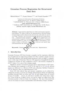
Fig. 1 nMSE of GPR on the 1st DOF under varying sample size. 1.014

1.01

1.01

1.008

1.008

1.006

1.006 1.004

500

700 900 Sample Size

1,100

10000

GPR

1.004 1.002

1.002

1

1 0

0.998 0

100

300

500

700 900 Sample Size

1,100

10000

Fig. 3 nMSE of GPR on the 3rd DOF under varying sample size. 1.035

100

300

500

700 900 Sample Size

1,100

10000

Fig. 4 nMSE of GPR on the 4th DOF under varying sample size. 1.34

GPR

1.03

GPR

1.335

1.025

1.33

1.02

1.325

nMSE

nMSE

300

1.012

GPR

1.012

1.015 1.01

1.32 1.315

1.005 1 0

100

Fig. 2 nMSE of GPR on the 2nd DOF under varying sample size.

nMSE

nMSE

1 0

10000

1.31 100

300

500

700 900 Sample Size

1,100

10000

Fig. 5 nMSE of GPR on the 5th DOF under varying sample size.

1.305 0

100

300

GPR

1.025

nMSE

1.02

1.015

1.01

100

300

500

700 900 Sample Size

700 900 Sample Size

1,100

10000

Fig. 6 nMSE of GPR on the 6th DOF under varying sample size.

1.03

0

500

1,100

10000

Fig. 7 nMSE of GPR on the 7th DOF under varying sample size.

Learning Inverse Dynamics by Multi-Task Gaussian Process Regression 1.1

1.1

1

1 GPR Multi−Task GPR

0.9

0.8 nMSE

nMSE

0.7

0.7

0.6

0.6

0.5

0.5 0.4

0.4 100

300

500

700 900 Sample Size

1,100

10000

Fig. 8 nMSE of Multi-Task GPR on the 1st DOF under varying sample size.

0

100

300

500

700 900 Sample Size

1,100

10000

Fig. 9 nMSE of Multi-Task GPR on the 2nd DOF under varying sample size.

1.1

1.4

1

1.2 GPR Multi−Task GPR

0.9

GPR Multi−Task GPR

1 nMSE

0.8 nMSE

GPR Multi−Task GPR

0.9

0.8

0

13

0.7

0.8 0.6

0.6 0.4

0.5

0.2

0.4 0

100

300

500

700 900 Sample Size

1,100

0 0

10000

Fig. 10 nMSE of Multi-Task GPR on the 3rd DOF under varying sample size.

1.6

1

1.55 GPR Multi−Task GPR

700 900 Sample Size

1,100

10000

GPR Multi−Task GPR

1.5

nMSE

nMSE

500

1.45

0.8 0.7

1.4 1.35

0.6 0.5

1.3

0.4

1.25

0

300

Fig. 11 nMSE of Multi-Task GPR on the 4th DOF under varying sample size.

1.1

0.9

100

100

300

500

700 900 Sample Size

1,100

10000

Fig. 12 nMSE of Multi-Task GPR on the 5th DOF under varying sample size.

0

100

300

1 GPR Multi−Task GPR

0.8 nMSE

0.7 0.6 0.5 0.4 0.3 0.2 0.1 0

100

300

500

700 900 Sample Size

700 900 Sample Size

1,100

10000

Fig. 13 nMSE of Multi-Task GPR on the 6th DOF under varying sample size.

1.1

0.9

500

1,100

10000

Fig. 14 nMSE of Multi-Task GPR on the 7th DOF under varying sample size.