Using modeling languages for the complementary suppression problem through network flow models Jordi Castro F. Javier Heredia Statistics and Operations Research Department Universitat Polit`ecnica de Catalunya Pau Gargallo 5, 08028 Barcelona (Spain)
[email protected] [email protected] DR 2001-03 January 2001
Report available from http://www-eio.upc.es/~jcastro
Using modeling languages for the complementary suppression problem through network flow models ∗ Jordi Castro † F. Javier Heredia ‡ Statistics and Operations Research Department Universitat Polit`ecnica de Catalunya Pau Gargallo 5, 08028 Barcelona
[email protected] [email protected]
Abstract Several network flows based methods have been suggested in the past for the solution of the complementary suppression problem (CSP). Adding some of those methods to the τ -Argus system is one of the tasks to be performed in the scope of the ongoing IST CASC project. In this paper the authors briefly present how modeling languages can be used for the quick development of algorithm prototypes for CSP. This will permit evaluating and testing different algorithmic options prior to the costly development of an efficient exploitation code. We illustrate the use of modeling languages with a particular network flow based method. This method is implemented using a state-of-the-art modeling language, and some preliminary computational results are presented.
Key words: Disclosure protection, complementary cell suppression, linear programming, network optimization, modeling languages.
1
Introduction
Network flows models have been widely used in the past to avoid the disclosure of sensitive cells of statistical tables (see [3] for a comprehensive description). However, the τ -Argus system developed in a previous ESPRIT project lacks of such a methodology. Adding it to τ -Argus is one of the tasks to be performed in the recently started IST CASC project. This paper presents the first steps performed to achieve this goal. In particular, we will show that, before developing a costly implementation, using a modeling language can be instrumental to see in practice the drawbacks and benefits of a particular approach. We will focus on an heuristic procedure ∗ Work
supported by the IST-2000-25069 CASC project. supported by CICYT Project TAP99-1075-C02-02. ‡ Author supported by CICYT Project TAP99-1075-C02-01. † Author
1
for multiple-cell suppression under a minimum-number-of-suppressions criterion, based on an optimal method for single-cell suppression. This approach is described in [3]. Alternative methods could be attempted and implemented using AMPL in a similar way. An additional benefit of using a modeling language is that trying and developing new algorithms is (usually) a straightforward task. For instance, it could be studied the behaviour of alternative approaches based on network flows with side constraints [6] or multicommodity flows [2], and how can they be applied to multiple dimensional and/or hierarchically related tables. It is worth to note that, unlike network flows based methods that only provide approximate solution, there are other approaches that solve the CSP optimally. For instance in [4] a branch-and-cut based procedure was presented for the efficient solution of large CSP instances. This methodology is already available in τ -Argus. Network flows based methods can be seen as a complementary tool that will provide the end-user of τ -Argus the option of choosing between different strategies. This paper is organized as follows. Section 2 briefly describes the simple network flows based method considered in this work. Section 3 presents the AMPL implementation of the method. Finally, Section 4 presents some preliminary results obtained in the solution of a set of 64 randomly generated instances.
2
A network flows based method for the CSP
We will focus on a simple network flows based method (see [3] for a thorough description). The method attempts to minimize the number of secondary suppression cells. When applied to a single primary suppression cell the method is optimum. However, for multiple primary suppression cells the method is applied iteratively, at maximum once for each primary suppression cell, and optimality is not guaranteed (instead, an upper bound to the minimum number of suppressions is obtained).
2.1
Protecting a single cell
Let’s consider a table [aij ], i = 1 . . . m, j = 1 . . . n, m being the number of rows and n the number of columns. Marginal total values are denoted as am+1,j , ai,n+1 and am+1,n+1 , where
ai,n+1 am+1,j am+1,n+1
= = =
n X j=1 m X i=1 n X
aij
i = 1...m
(1)
aij
j = 1...n
(2)
am+1,j =
j=1
m X
ai,n+1 .
(3)
i=1
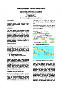
The above linear relations can be modeled through a directed graph G = (V, A), V being a set of m + n + 2 nodes and A a set of (m + 1)(n + 1) arcs. Figure 1 shows the structure of G. There is one node for each row and column 2
Figure 1: Representation of a table as a directed graph. 1
1
2
2 m+1
. . .
. . .
n+1
m
n
of the table (nodes 1 . . . m and 1 . . . n of Figure 1), plus two additional nodes for the row and column totals (nodes n+1 and m+1 of Figure 1, respectively). Cells aij , 1 ≤ i ≤ m, 1 ≤ j ≤ n are related to arcs (i, j). Row totals cells ai,n+1 , 1 ≤ i ≤ m are related to arcs (n + 1, i), while column totals cells am+1,j , 1 ≤ j ≤ n correspond to arcs j, m + 1. Total cell am+1,n+1 is related to arc (m + 1, n + 1). Given a set S = {(i1 , j1 ), . . . , (ip , jp )} of p suppression cells, one can optimally protect under the minimum-number-of-suppressions criterion a particular target cell (it , jt ), 1 ≤ t ≤ p solving a network flows problem. This problem is defined over the graph G 0 = (V, A0 ), where A0 = {(i, j), (j, i)|(i, j) ∈ A} (i.e., we have in A0 a forward and reverse arc for each arc of Figure 1). For each arc in A0 we consider one variable, denoted as x+ ij if the origin arc corresponds either to a row node or to the column total node m + 1 (i.e., (i, j), i = 1, 2, . . . , m + 1, j = 1, 2, . . . , n + 1) and x− ij if the origin arc corresponds either to a column node or to the row total node n + 1 (i.e., (i, j), i = 1, 2, . . . , n + 1, j = 1, 2, . . . , m + 1) . Default lower and upper bounds are respectively 0 and 1 for the 2(m + 1)(n + 1) variables. Node injections are zero. Since bounds and injections are integer, it is guaranteed that the solution of any defined network flows problem will be integer as well [1] (in this case, it will be a pattern of 0-1 flows). Moreover, since we consider zero injections at nodes, the optimal solution of any problem defined over this network will be either 0 for all the variables, or —should we forced a positive flow— a 1 flow for some arcs forming a cycle C in A0 . It can be shown that the target cell (it , jt ) will be protected if the optimal solution of the network flows problem is a nontrivial cycle C in A0 such that (it , jt ) ∈ C. By nontrivial cycles we mean cycles with a number of arcs ≥ 4, − thus avoiding spurious solutions as x+ it ,jt = xit ,jt = 1 and 0 for the remaining variables. This can be guaranteed by imposing an upper bound of 0 to variable + − x− it ,jt . The rest of xij or xij variables of the cycle correspond to (i, j) cells that need to be suppressed to protect cell (it , jt ). Then, in order to minimize the number of suppressions, cells of S have to be used whenever possible before including additional complementary ones. This is guaranteed if the following cost vector is used during the optimization of the network flows problem:
3
−(C + 1) if (i, j) = (it , jt ) 1 if (i, j) ∈ S, (i, j) 6= (it , jt ) c+ ij = |S| if (i, j) 6∈ S, ½ 1 if (i, j) ∈ S − cij = |S| if (i, j) 6∈ S,
(4)
(5)
where |S| is the cardinality of S, and C=
X
− (c+ ij + cij ) = 2[((m + 1)(n + 1) − |S|)|S| + 2(|S| − 1)].
(6)
(i,j)6=(it ,jt )
This cost vector forces to set x+ it ,jt = 1 due to its large negative cost. Variables associated with cells in S will also be used before adding any complementary suppression cell. The solution of this problem provides an optimal solution for the protection of the single cell (it , jt ) under the minimum-numberof-suppressions criterion.
2.2
Protecting multiple cells
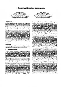
The protection of multiple cells can be accomplished by iteratively applying the procedure described in previous section. This heuristic procedure will provide an upper bound instead of the optimum number of secondary suppressions, as noted in [3]. Figure 2 shows the main steps of a naive algorithm based on this idea. The parameters of the algorithm are a table and a set of primary suppressions denoted by S0 , possibly ordered by descending importance. SP, the set of protected cells, is initially equal to the empty set. At each iteration of the algorithm we choose the next target cell of S0 not yet protected (line 3). The protection of the target cell is performed through the network flows problem of previous subsection (line 4). The set S to be used for the definition of the costs (4) and (5) is Sk , which is modified at each iteration of the algorithm. The cycle of the optimal solution corresponds to those cells that were protected by the network flows problem. Some of them will already be in Sk . The rest are complementary suppressions, which are added to Sk+1 and the set of protected cells SP. The algorithm iterates until Sk is equal to SP, i.e., all the primary suppressions of S0 are protected. Note that, at most, one network flows problem needs to be performed for each primary suppression cell of S0 . Although this algorithm could be improved with additional refinements, its current form will be enough to show how a modeling language can be used for a quick implementation.
3
The AMPL model
We chose the AMPL modeling language [5] for the implementation of the single and multiple-cell suppression problems of subsections 2.1 and 2.2. This is one of the most versatile modeling languages currently available, permitting, among other features, implementing iterative procedures (as that of Figure 2) and solving the resulting optimization problems through a high variety of packages (including own routines). Moreover, there are specialized servers in Internet (e.g., 4
Figure 2: Multiple-cell protection heuristic procedure. Algorithm Multiple-cell protection(Table,S0 ): 1 SP := ∅, k := 0; 2 while Sk 6= SP do 3 Find next target cell (it , jt ) ∈ S0 such that (it , jt ) 6∈ SP; 4 Solve network flow problem of subsection 2.1 for S := Sk ; 5 Obtain cycle C of the optimal solution; 6 SP := SP ∪ C; 7 Sk+1 := Sk ∪ C ; 8 k := k + 1; 9 end while End algorithm
http://www-neos.mcs.anl.gov/neos) that freely permit the remote solution of problems formulated in the AMPL language [8]. Briefly, to implement the CSP algorithms of previous sections through AMPL we need: • A .dat file with the data of the particular instance to be solved (table, and set of primary suppression cells). • A .run file with the description of the iterative algorithm, i.e., the multiplecell protection heuristic of Figure 2. • A .mod file with the description of the network flows problems of subsection 2.2 to be solved at each iteration. Although we won’t enter into details, it is worth to include the code of the above files to see how straighforward is an AMPL implementation (see Figures 3–5 of Appendix A). Figure 3 shows the data for a particular instance made of a table 3 × 4 and 2 primary suppression cells —(1, 1) and (2, 2). Figures 4 and 5 show all the code required to implement respectively the iterative procedure and the network flows problems. Note that only 72 lines of code were required. This permits easily trying alternative algorithmic options (new heuristics, different costs—with the inclusion of cells values—, alternative solvers, etc.) before developing a final explotation code.
4
Computational results
We tested the AMPL implementation of the previous section with a set of 64 randomly generated problems. Each instance depends of three parameters (m, n, p), which denote the number of rows, columns and primary suppressions, respectively. The p primary cells were randomly distributed inside the table. The 64 instances were obtained considering all the combinations for m, n, p ∈ {50, 100, 150, 200}. 5
Table 1: Results for the 64 randomly generated problems m 50 50 50 50 50 50 50 50 50 50 50 50 50 50 50 50 100 100 100 100 100 100 100 100 100 100 100 100 100 100 100 100
n 50 50 50 50 100 100 100 100 150 150 150 150 200 200 200 200 50 50 50 50 100 100 100 100 150 150 150 150 200 200 200 200
p 50 100 150 200 50 100 150 200 50 100 150 200 50 100 150 200 50 100 150 200 50 100 150 200 50 100 150 200 50 100 150 200
|SP| 95 135 162 203 90 145 184 233 101 168 219 255 104 172 225 272 101 148 194 234 97 181 226 254 99 183 260 284 108 197 261 310
6
NFP 33 42 47 71 29 47 62 85 35 61 76 86 35 61 78 94 37 50 65 80 31 63 76 78 30 59 89 86 33 65 89 105
CPUNF 2.04 2.69 3.04 4.54 3.68 6.09 8.14 11.19 6.97 12.19 15.35 17.41 9.42 16.53 21.40 25.91 4.75 6.75 8.65 10.78 8.28 17.16 20.92 21.47 12.66 24.96 37.33 36.88 19.16 37.90 52.16 62.27
Table 1(cont.): Results for the 64 randomly generated problems m 150 150 150 150 150 150 150 150 150 150 150 150 150 150 150 150 200 200 200 200 200 200 200 200 200 200 200 200 200 200 200 200
n 50 50 50 50 100 100 100 100 150 150 150 150 200 200 200 200 50 50 50 50 100 100 100 100 150 150 150 150 200 200 200 200
p 50 100 150 200 50 100 150 200 50 100 150 200 50 100 150 200 50 100 150 200 50 100 150 200 50 100 150 200 50 100 150 200
|SP| 98 160 212 260 99 180 233 278 102 189 264 317 105 196 265 342 97 176 225 279 101 181 254 304 107 204 277 335 110 214 282 354
7
NFP 33 56 76 91 30 56 75 88 31 62 91 104 32 60 87 119 32 64 78 99 30 60 87 102 34 67 91 112 32 67 88 116
CPUNF 6.50 11.44 15.51 18.48 12.48 23.48 31.91 38.34 20.85 41.43 61.00 73.54 29.16 54.94 80.64 13.29 8.73 17.60 22.12 28.02 18.03 36.06 53.28 66.61 31.74 62.58 85.49 107.62 41.30 86.70 113.93 151.85
Table 1 shows the results obtained. Executions were performed on a Sun Ultra2 200MHz workstation, of ≈68 Linpack Mflops, 14.7 Specfp95 and 7.8 Specint95 (this machine is approximately equivalent to a 350 Mhz Pentium PC). Columns m, n and p have the meaning above described. Column |SP| gives the final number of (primary plus secondary) suppressions obtained by the heuristic procedure. Column NFP shows the number of network flow subproblems solved. Finally, column CPUNF gives the CPU time spent by the code in the solution of the network flows problems. They were solved using the state-of-the-art network solver of the Cplex 6.5 package [7]. The execution time of the overall procedure is not presented because it is meaningless: AMPL is not a compiled language, thus executions are fairly large. In an efficient C implementation the overall execution time should be close to that of the CPUNF column. No computational results were presented in [3] for a similar approach, so the results obtained can not be compared with those of previous implementations. It is worth to note that these results have been obtained with a naive heuristic procedure, thus it should be possible to improve them. However, although the number of network flow problems solved is fairly less than p —the number of primary cells—, their solution still requires a significant computational effort. Moreover, this effort increases with p. Even with alternative network solvers [9], for large instances, this procedure could be very expensive. In this case, a quickly developed AMPL model has been enough to understand the main drawbacks of this approach, avoiding a costly C implementation of the algorithm.
5
Conclusions
The main concern of this paper has been to show how modeling languages as AMPL could be used to obtain easy and quick (although not efficient) prototype implementations. As an example, the AMPL code for the heuristic procedure of Cox [3] for CSP has been presented. This prototype implementation has been used to solve a set of randomly generated problems ranging from m = 50, n = 50 and 50 primary cells to m = 200, n = 200 and 200 primary cells. Developing and testing additional networks based methods, and implementing for τ -Argus those that eventually appear to be efficient, is part of the further work to be done.
References [1] R.K. Ahuja, T.L. Magnanti and J.B. Orlin, Network Flows, Prentice Hall, Englewood Cliffs, NJ, 1993. [2] J. Castro, A specialized interior-point algorithm for multicommodity network flows, SIAM J. on Optimization 10(3), pp. 852–877, 2000. [3] L.H. Cox, “Network models for complementary cell suppression”, J. of the American Statistical Association 90, pp. 1453–1462, 1995. [4] M. Fischetti and J.J. Salazar, “Models and algorithms for the 2-dimensional cell suppression problem in statistical disclosure control”, Mathematical Programming 84, pp. 283–312, 1999.
8
[5] R. Fourer, D.M. Gay and B.W. Kernighan, AMPL: A Modeling Language for Mathematical Programming, Duxbury Press, 1993. [6] F.J. Heredia and N. Nabona, “Numerical implementation and computational results of nonlinear network optimization with linear side constraints”. P. Kall (Ed.). System Modelling and Optimization. Proceedings of the 15th IFIP Conference, Springer-Verlag, pp. 301–310, 1991. [7] ILOG CPLEX, ILOG CPLEX 6.5 Reference Manual Library, ILOG, 1999. [8] J. Czyzyk, M. Mesnier and J. Mor´e, “The NEOS Server”, IEEE Journal on Computational Science and Engineering, 5, pp. 68–75, 1998. [9] M.G.C. Resende and G. Veiga, “An implementation of the dual affine scaling algorithm for minimum cost flow on bipartite uncapacitated networks”, SIAM J. on Optimization, 3, pp. 516–537, 1993.
A
AMPL files Figure 3: AMPL .dat code for a particular instance. param m param n param p param: 1 2 param a 1 2 3 4
:= 3; := 4; := 2; p_r 1 2 : 1 1 500 297 798
p_c := 1 2 ;
2 111 1 143 255
3 172 9 212 393
9
4 165 256 184 605
5 := 449 766 836 2051 ;
Figure 4: AMPL .run code for the iterative procedure. model csp.mod; data csp_instance.dat; option solver cplex65; param i_p; let S0 := {}; for {i in 1..p}{ let S0:= S0 union {(p_r[i],p_c[i])}; } let S := S0; let i_p := 1; let TARGET := {(p_r[i_p],p_c[i_p])}; let Sprot :={}; let CYCLE :={}; problem Nc: Num_CS, Xpos, Xneg, Row, Column; repeat { solve Nc; let CYCLE := {}; for {(i,j) in (LINKS)} { if Xpos[i,j]>0.99 or Xneg[i,j]>0.99 then{ let CYCLE := CYCLE union {(i,j)}; } } let S := S union CYCLE; let Sprot := Sprot union CYCLE; if card(S) != card(Sprot) then { repeat { let i_p:= i_p + 1; } until (p_r[i_p],p_c[i_p]) not in Sprot; let TARGET := {(p_r[i_p],p_c[i_p])}; } else { let TARGET:={}; let i_p := 0; } } until card(Sprot) == card(S);
10
Figure 5: AMPL .mod code for the network flows problems. param m integer >0 ; #number of rows (without totals row) param n integer >0 ; #number of columns (without totals column) param p integer >0; #number of primary suppression cells param p_r{1..p} integer, >=1, =1, = (if (i,j) in TARGET then 1 else 0), =0,