Using motion primitives in probabilistic sample-based planning for ...

Using motion primitives in probabilistic sample-based planning for humanoid robots Kris Hauser1 , Tim Bretl1 , Kensuke Harada2 , and Jean-Claude Latombe1 1

2

Computer Science Department, Stanford University {khauser,tbretl}@stanford.edu and [email protected] National Institute of Advanced Industrial Science and Technology (AIST) [email protected]

Abstract: This paper presents a method of computing efficient and natural-looking motions for humanoid robots walking on varied terrain. It uses a small set of highquality motion primitives (such as a fixed gait on flat ground) that have been generated offline. But rather than restrict motion to these primitives, it uses them to derive a sampling strategy for a probabilistic, sample-based planner. Results in simulation on several different terrains demonstrate a reduction in planning time and a marked increase in motion quality.

1 Introduction In this paper we present a method of planning efficient and natural-looking motions for humanoid robots on varied terrain. One thing that makes this problem difficult is that although humanoids have many degrees of freedom (dof), we do not know in advance which of these dof are actually useful, nor which contacts may be needed. On easy terrain like flat ground or stairs of fixed height, the motion of a humanoid is lightly constrained, most of its dof are redundant, and only feet need contact the ground. On hard terrain like steep rock or urban rubble, the motion of a humanoid is highly constrained, most of its dof are essential, and additional contacts (hands, knees, shoulders) might be required for balance. On varied terrain, the number of relevant dof and the types of required contacts may change from step to step. Consequently, planners that simplify the problem by considering a subset of the robot’s dof work well on easy terrain, but are not flexible enough to handle varied terrain. For example, one strategy for a humanoid on mostly flat ground is to precompute a library of feasible steps [22]. Each step is a continuous trajectory that places one foot in a new location relative to the other. Motions are constructed as a sequence of these steps. Because this only requires searching a graph, rather than a high-dimensional configuration space, it can be done quickly. More importantly, because the steps are precomputed, the resulting motion is efficient and robust, and looks natural. However, when

2

Kris Hauser, Tim Bretl, Kensuke Harada, and Jean-Claude Latombe

the ground is not flat – in particular, when hands are required for balance – this approach may not be able to find a feasible motion. Conversely, planners that consider all of the robot’s dof work well on hard terrain, but do not generate efficient or natural-looking motions (when this is possible) on varied terrain. For example, one strategy for a humanoid on severely uneven ground (based on earlier work for a free-climbing robot [5]) begins by identifying a number of potentially useful contacts [16]. Each mapping of hands or feet to contacts is a stance, associated with a (possibly empty) set of feasible configurations that satisfy all motion constraints. The robot can take a step from one stance to another if they differ by a single contact and if they share a feasible configuration, called a transition. The planner proceeds in two stages: first, it generates a candidate sequence of contacts by finding transitions between stances; then, it refines this sequence into a feasible, continuous trajectory by finding paths between subsequent transitions. Probabilistic, sample-based algorithms are used to find both transitions and paths. This approach is fast on irregular and steep terrain, because in this situation the robot’s motion is most constrained just as it makes or breaks a contact. But when the ground is flat, this approach takes longer than the one of [22], and may generate needless motions of the arms or other dof that are not required for balance. These motions are hard to eliminate in post-processing. Rather than select one approach or the other, our planner combines the strengths of both. First, we generate a small set of high-quality motion primitives (similar to [22]), that might include a single step on flat ground, or an arm movement that places a hand on a wall for balance. Here, these primitives are produced by a lengthy off-line precomputation, but they might also be designed by hand or even captured or learned from examples of human motion. We record each motion primitive as a nominal path through the robot’s configuration space (a joint-angle trajectory). Then, we use the two-stage strategy of [5, 16] to plan motions of the humanoid on-the-fly. But instead of sampling across all of configuration space to find transitions between stances and paths between transitions, we sample in a growing distribution around the nominal path associated with a chosen motion primitive. Although still preliminary, our simulation results demonstrate a reduction in planning time and a marked increase in motion quality3 for a humanoid walking on varied terrain.

2 Related work Motion primitives and other types of maneuvers have been applied widely to robotics and digital animation. Four general strategies have been used: Record and playback. This strategy restricts motion to a library of maneuvers. Natural-looking humanoid locomotion on mostly flat ground can be planned as a sequence of precomputed feasible steps [22]. Robust helicopter flight can be 3

Exactly how motion quality should be measured is an open question, beyond the scope of this paper. Here, we define quality as inversely proportional to a linear combination of path length and sum-squared distance from an upright posture.

Motion primitives in probabilistic sample-based planning

3

planned as a sequence of feedfoward control strategies (learned by observing skilled human operators) to move between trim states [10–12, 31]. Robotic juggling can be planned as a sequence of feedback control strategies [8]. The motion of peg-climbing robots can be planned as a sequence of actions like “grab the nearest peg” [3]. In these applications, a reasonably small library of maneuvers is sufficient to achieve most desired motions. For humanoid robots on varied terrain, such a library may grow to impractical size. Warp, blend, or transform. Widely used for digital animation, this strategy also restricts motion to a library of maneuvers, but allows these maneuvers to be superimposed or transformed to better fit the task at hand. For example, captured motions of human actors can be “warped” to allow characters to reach different footfalls [40] or “retargetted” to control characters of different morphologies [13]. Of course, for a digital character it is most important to look good while for a humanoid robot it is most important to satisfy hard motion constraints. So although some techniques have been proposed to transform maneuvers while maintaining physical constraints [34, 39], this strategy seems better suited for animation than robotics. Model reduction. This strategy plans overall motion first, following this motion with a concatenation of primitives. For example, another way to generate natural-looking humanoid locomotion on flat ground is to approximate the robot as a cylinder, plan a 2-d collision-free path of this cylinder, and follow this path with a fixed gait [19–21, 32]. A similar method is used to plan the motion of nonholonomic wheeled vehicles [23, 24]. A related strategy plans the motion of key points on a robot or digital actor (such as the center of mass or related ground reference points [33]), tracking these points with an operational space controller [38]. These approaches work well when it does not matter much where a robot or digital actor contacts its environment. When the choice of contact location is critical, as is often the case for humanoids on varied terrain, it makes more sense to compute a sequence of footfalls first. Bias inverse kinematic solutions. Like model reduction, this strategy first plans the motion of key points on a robot or digital actor, such as the location of hands or feet. But instead of a fixed controller, a search algorithm is used to compute a pose of the robot or actor at each instant that tracks these points (an inverse kinematic solution). One approach is to choose an inverse kinematic solution according to a probability density function learned from high-quality example motions [15, 28, 29, 41]. The set of examples give the resulting pose a particular “style.” In fact, we take a similar approach in this paper, planning steps for a humanoid by sampling waypoints in a growing distribution around high-quality nominal paths.

3 Background Our planner extends a similar one for humanoid robots [16], which was based on earlier work for a free-climbing robot [5]. Here, we summarize our basic approach and describe the limitations we address by using motion primitives.

4


(a)

(b)

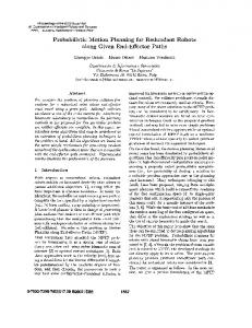
Fig. 1. (a) The humanoid robot hrp-2 [18]. (b) Example of varied terrain.

3.1 Motion constraints We consider the humanoid hrp-2 (Fig. 1(a)). A configuration q consists of 6 parameters defining the position and orientation of the torso and a list of 30 revolute joint angles. The set of all such q is the configuration space, denoted Q, of dimensionality 36. We consider terrain that might include a mixture of flat, sloped, or rocky ground (Fig. 1(b)). We assume that this terrain and all robot links are perfectly rigid. We also assume that we are given in advance a set of links (such as hands, feet, or knees) that are allowed to touch the terrain. We call the placement of a link on the terrain a contact, and fix the position and orientation of the link while the contact is maintained. We call a set of simultaneous contacts a stance, denoted by σ. Consider a stance σ with n ≥ 1 contacts. The feasible space Fσ is the set of all feasible configurations of the robot at σ. To be in Fσ , a configuration q must satisfy several constraints: Contact. The n contacts form a linkage with multiple closed-loop chains, so q must satisfy inverse kinematic equations. Let Qσ ⊂ Q be the set of all configurations q that satisfy these equations. This set is a possibly empty submanifold of Q of dimensionality 36 − 6n, which we call the stance manifold. Equilibrium. To balance at a fixed stance σ, hrp-2 must apply forces at contacts in σ that compensate for gravity without slip. For valid forces to exist, hrp-2’s center of mass (cm) must lie above its support polygon. On varied terrain, this polygon does not always correspond to the base of hrp-2’s feet [5–7]. So we model each contact as a set of frictional points, and compute the support polygon as in [6,16]. When the cm lies above this polygon, we also check that joint torques achieving the required contact forces are within bounds. Collision. In addition to satisfying joint angle limits, the robot must avoid collision with the environment (except at contacts) and with itself [14, 37]. 3.2 Motion planning We assume hrp-2 moves from one place to another by taking a sequence of steps. Each step is a continuous motion at a fixed stance that ends by


5

making or breaking a single contact. In particular, suppose the robot begins at a configuration q ∈ Fσ at a stance σ. A single step from q consists of three parts: first, a contact that is made or broken to move from σ to a new stance σ 0 ; second, a configuration q 0 ∈ Fσ ∩ Fσ0 , which we call a transition, that is feasible at both σ and σ 0 ; third, a feasible path in Fσ from q to q 0 . Following the approach of [5, 16], we make these three choices hierarchically. To find a contact, we randomly sample potential placements of the robot’s links in the terrain (or select a placement in σ to release). We use heuristics to decide which placement is most likely to lead toward the goal. To find a transition given σ 0 , we randomly sample configurations in Qσ (or in Qσ0 if σ ⊂ σ 0 ) and reject them if they are not in Fσ ∩ Fσ0 . We use the combination of a bounding-volume technique similar to [9] and an iterative Newton-Raphson method to sample configurations in Qσ (which has zero measure in Q). To find a path given q 0 , we use a variant of the probabilistic roadmap (prm) algorithm called sbl [36]. This algorithm is bidirectional (growing trees, as in [25], from both q and q 0 ) and lazy (delaying the creation of local paths until a candidate sequence of milestones is found). 3.3 Current limitations Our search strategy postpones finding one-step paths (a costly computation) until after finding transitions and contacts [5, 16]. It works well for hrp-2 on irregular and steep terrain because in this situation, the robot’s motion is most constrained just as it makes or breaks a contact. In particular, we have observed in our experiments that if q ∈ Fσ ∩ Fσ0 and q 0 ∈ Fσ ∩ Fσ00 exist, then a path between q and q 0 in Fσ likely also exists. However, because we randomly sample each transition and use prm to plan each one-step path, the motions we generate are feasible (given an accurate terrain model) but not necessarily high-quality. For example, when hrp-2 walks on terrain that is not irregular and steep, its motion is lightly constrained. Each step we generate might contain strange or erratic motions of the arms and legs. These motions are difficult to eliminate in post-processing. Also, because we randomly sample each contact, we might end up trying difficult steps when simpler ones would have led to the goal as well. For example, the robot might reach a stance σ associated with a feasible space Fσ containing a narrow passage. With only a small perturbation of the contacts at σ, this narrow passage is likely to disappear [17]. So although additional steps might still be possible, they would be easier to compute if we had made a better choice of contacts at σ.

4 Generating motion primitives We address the limitations of our planner by using a library of motion primitives. Each primitive is a single step of very high quality. In this section, we describe how we generate primitives. In the following section, we will describe how they guide our selection of paths, transitions, and contacts.

6


(a)

(b)

Fig. 2. Two primitives on flat ground, to (a) place a foot and (b) remove a foot. The support polygon – here, just the convex hull of supporting feet – is shaded blue.

Currently, it is the responsibility of the user to decide which primitives to include in the library. First, we need to identify a small but representative set of steps to be learned and to specify start and goal stances (differing by a single contact) for each one. These steps should be both important (often repeated) and broadly applicable (similar to a wide variety of other steps). For example, we might choose to include several consecutive steps on flat ground, each placing or removing a foot (Fig. 2). Next, we need to define a weighted set of criteria to judge the quality of each step. For example, we might choose to minimize path length, torque, energy, or the amount of deviation from an upright posture. Finally, we need to decide whether to accept or reject a candidate primitive, because we are not guaranteed that our optimization criteria correspond to our aesthetic notion of what is “natural.” It is the responsibility of the planner to actually compute each primitive. First, we generate an initial trajectory between the given start and goal stances by randomly sampling a feasible transition and creating a path to reach it using prm, as in [5, 16]. Then, we optimize this trajectory with respect to the given objective function using a standard nonlinear optimization package [26]. This entire process is an off-line precomputation; several hours were required to generate the two example primitives in Fig. 2. The generation of motion primitives has not been the main focus of our work (this paper concerns their application to planning), so many improvements may be possible. For example, we expect better results to be obtained by using the method of optimization proposed by [4]. Likewise, we might use a learned classifier to decide (without supervision) whether candidate primitives look natural, as in [35]. Finally, we might automate the selection of primitives to include in our library by learning a statistical model of importance (similar


7

to location-based activity recognition [27]) or applicability after perturbation (similar to prm planning with model uncertainty [30]). We record each primitive in our library as a nominal path u : t ∈ [0, 1] → u(t) ∈ Q in configuration space that does one of two things: • Adds a contact. For some σ and σ 0 such that σ ⊂ σ 0 , u is a feasible path in Fσ from u(0) ∈ Fσ to u(1) ∈ Fσ ∩ Fσ0 . • Removes a contact. For some σ and σ 0 such that σ ⊃ σ 0 , u is a feasible path in Fσ from u(0) ∈ Fσ to u(1) ∈ Fσ ∩ Fσ0 . We will denote the start and goal stances for each primitive u by σu and σu0 , respectively. In general, u will only define a feasible step between σu and σu0 , but we will see in the next section that it can still be used to help guide our choice of path, transition, and contact to reach other stances.

5 Using primitives for planning We use motion primitives to help our planner generate each step. We do this at three levels: finding a path (given a transition and a final stance), finding a transition (given only the final stance), and finding a contact (in order to define the final stance). In each case, first we transform the primitive to better match the step we are trying to plan, then we apply the transformed primitive to bias the sampling strategy used by our planner. 5.1 Finding paths Consider the robot at an initial configuration qinitial ∈ Fσ at an initial stance σ. Assume that we are given a final stance σ 0 and a transition qfinal ∈ Fσ ∩ Fσ0 (recall qfinal is a configuration feasible at both σ and σ 0 ). Also assume that we are given an appropriate primitive u ⊂ Q (as described in Section 4). We want to use u to guide our search for a path from qinitial to qfinal in Fσ . As before, we use sbl (a variant of prm) to grow trees from root configurations [36]. But rather than root these trees only at qinitial and qfinal , we root them at additional configurations (similar to [1]) sampled according to the primitive u. Transforming the primitive to match qinitial and qfinal . Although we assume u is similar to the step we are trying to plan, it will not be identical. So first, we transform u so that it starts at qinitial and ends at qfinal . We have chosen to use an affine transformation of the form u ˆ(t) = A (u(t) − u(0)) + qinitial

(1)

that maps the straight-line segment between u(0) and u(1) to the segment between qinitial and qfinal . In other words,

8

Kris Hauser, Tim Bretl, Kensuke Harada, and Jean-Claude Latombe nominal path u u(1)

q2 q4

u(0) transformed path u ˆ

q1 (qinitial )

q3 qˆ4

qinitial

q5 (qfinal ) qfinal

(a)

(b)

q2

q1

q3 q4 q5

(c)

(d)

Fig. 3. Using a primitive to guide path planning. (a) Transforming a motion primitive to start at qinitial and end at qfinal . (b) Sampling root milestones in Fσ near equally spaced waypoints along u ˆ. (c) Growing trees to connect neighboring roots. (d) The resulting path, which if possible is close to u ˆ (dotted).

u ˆ(0) = A (u(0) − u(0)) + qinitial = 0 + qinitial = qinitial

u ˆ(1) = A (u(1) − u(0)) + qinitial = (qfinal − qinitial ) + qinitial = qfinal

In particular, we select A closest to the identity matrix, minimizing X min (Aij − δi,j )2 such that A (u(1) − u(0)) = qfinal − qinitial A

i,j

where δij = 1 if i = j and 0 otherwise. We compute A in closed form as T

A=I+

((qfinal − qinitial ) − (u(1) − u(0))) (u(1) − u(0)) . ku(1) − u(0)k22

We can visualize this transformation as in Fig. 3(a). First, u is translated to start at qinitial . Then, the farther we move along u (the more we increase t), the closer u ˆ is pushed toward the segment from qinitial to qfinal .


9

Sampling root milestones. Let q1 , . . . , qn be configurations evenly distributed along u ˆ from qinitial to qfinal (Fig. 3(b)). For each i = 1, . . . , n, we test if qi ∈ Fσ . If so, we add qi as a root milestone in our roadmap. If not, we repeatedly sample other configurations in a growing neighborhood of qi until we find some feasible qi0 ∈ Fσ , which we add as a root instead of qi . Connecting neighboring roots with sampled trees. For i = 1, . . . , n − 1, we check if the root milestone qi can be connected to its neighbor qi+1 with a feasible local path (as in [16]). If not, we add the pair of roots (qi , qi+1 ) to a list R. Then, we apply prm to grow trees between every pair in R. For example, in Fig. 3(c) we add (q2 , q3 ) and (q4 , q5 ) to R and grow trees to connect both q2 with q3 and q4 with q5 . We process all trees in parallel. So at every iteration, for each pair (qi , qi+1 ) ∈ R, we first add m milestones to the trees at both qi and qi+1 (in our experiments, we set m = 5). Then, we find the configurations q connected to qi and q 0 connected to qi+1 that are closest. If q and q 0 can be connected by a local path, we remove (qi , qi+1 ) from R. When we connect all neighboring roots, we return the resulting path; if this does not happen after a fixed number of iterations, we return failure. Just like our original implementation, this approach will find a path between qinitial and qfinal whenever one exists (given enough time). However, since we seed our roadmap with milestones that are close to u, we expect the resulting motion to be similar (and of similar quality) to this primitive whenever possible (Fig. 3(d)), deviating significantly from it only when necessary. 5.2 Finding transitions Again consider the robot at a configuration qinitial ∈ Fσ at a stance σ. But now, assume that we are only given a final stance σ 0 , so we use a primitive u to guide our search for a transition before we plan a path to reach it. Transforming the primitive to match σ and σ 0 . Since we do not know qfinal , we can not use the same transformation (1) that we used for planning paths. Instead, we choose a rigid-body transformation of the form u ˆ(t) = Au(t) + b σu0

(2)

(associated with the primitive u) that maps the nominal stances σu and as closely as possible to the stances σ and σ 0 . Recall that a stance consists of several contacts, each placing a link of the robot on the terrain. If we model the surface of the terrain and all robot links as a triangular mesh, then we can define the location of each placement by a finite number of points ri ∈ R3 . For example, the face-face contact between a foot and the ground might be defined by the vertices r1 , r2 , and r3 of a triangle. We consider these points to be attached to the robot, so if the foot is placed against a different face in the terrain, the points r1 , r2 , and r3 move in R3 but remain in the same location relative to the foot. We will use these points to define our mapping between stances. In particular, let ri ∈ R3 for i = 1, . . . , m be the set of all points defining the contacts in both σu and σu0 , and let si ∈ R3 for i = 1, . . . , m be the set

10


of all points defining the contacts in both σ and σ 0 . (We assume u has been chosen so that both sets have the same number of points.) Then we choose the rotation matrix A and translation b in (2) that minimize X min kAri + b − si k22 . A,b

i

We can compute A and b in closed form [2]. But, we only consider rotations A about the gravity vector to avoid tilting the robot into an unstable orientation. Sampling a transition. As before, we sample configurations q ∈ Qσ , keeping them if q ∈ Fσ ∩ Fσ0 . But rather than sample configurations completely at random, we sample them in a growing neighborhood of u ˆ(1). We expect a well-chosen transition to further improve the quality of the path to reach it. 5.3 Finding contacts Once more, consider the robot at a configuration qinitial ∈ Fσ and a stance σ. But now, assume we are given neither a final stance nor a transition, but only a primitive u. If u removes a robot link from the terrain, we immediately generate a final stance σ 0 by removing the corresponding contact from σ. But if u places a link in the terrain, we use it to guide our search for a new contact. Transforming the primitive to match σ. We use the same transformation (2) to construct u ˆ as for finding transitions. But here, we compute A and b to map only σu to σ, since we do not know σ 0 . We use this transformation to adjust the placement of the new contact given by u. Let ri ∈ R3 for i = 1, . . . , m be the set of points defining this contact. Then the transformed contact is given by rî = Ari + b for i = 1, . . . , m. P Sampling a contact. We define a sphere of radius δ, centered at (1/m) i rî . We increase δ until the intersection of this sphere with the terrain is nonempty (initially, we set δ approximately the size of hrp-2’s foot). We randomly sample a placement of the points rî on the surface of the terrain inside the sphere, by first sampling a position of their centroid s ∈ R3 on the surface, then sampling a rotation of rî about the surface normal at s. We check that the contact defined by this placement has similar properties (normal vector, friction coefficient) to the contact defined by u. If so, we add it to σ to form σ 0 . If not, we reject it and sample another placement. 5.4 Deciding which primitive to use It only remains to decide which primitive u should be used, given an initial stance σ and configuration qinitial . We have experimented with a variety of heuristics. For example, we might pick the primitive that most closely matches σu with σ (in other words, that minimizes the error in a transformation of the form (2)). Likewise, we might pick the primitive that most closely matches σu0 with the actual terrain. However, the best approach is still not clear, and this issue remains an important area for future work.


11

6 Results An example of climbing a single stair. With each additional part of a step that we compute using a primitive, we add to the quality of the result. For example, consider the motion of hrp-2 in Fig. 4 to climb a single stair of height 0.3m (just below the knee). This motion was planned from scratch, by randomly sampling contacts and transitions and by using prm to generate paths. The robot does not look natural – its arm and leg motions are erratic, and its step over the stair is needlessly long. To improve this motion, we applied the two primitives shown in Fig. 2 (steps on flat ground). Fig. 5 shows the result of using these primitives to plan each path. Some erratic leg motions are eliminated, such as the backward movement of the leg in the second frame. The erratic arm motions remain, however, because the transition in the fourth frame is the same (still randomly sampled). Fig. 6 shows the result of using primitives to adjust this transition as well as to plan paths, eliminating most of the erratic arm motions. Finally, Fig. 7 shows the result of using primitives to select contacts well as plan transitions and paths. The chosen contact resulted in a much easier step, eliminating the extreme lean in the fifth frame. Planning time and motion quality for stairs of different heights. In our experiments, we have observed that planning time remains low and motion quality remains high even when we use a primitive to plan a step that is quite different. For example, we adapted the same two primitives in Fig. 2 to stairs of height 0.2m and 0.4m as well as 0.3m. Fig. 8 shows the results, averaged over five runs. Quality is measured by an objective function that penalizes both path length and deviations from an upright posture (lower values indicate higher quality). For comparison, we report the minimum objective value achieved after a lengthy off-line optimization. These results demonstrate that our use of primitives provides a modest reduction in planning time but significantly improves motion quality. Note also that both time and quality degrade gracefully as the step we are planning deviates further from the primitive. A variety of other examples. We have tested our planner in many other example environments. Fig. 9 shows hrp-2 on uneven terrain (using the primitives in Fig. 2), in which the highest and lowest point differ by 0.5m. Fig. 10 shows hrp-2 climbing a ladder with rungs that have non-uniform spacing and that deviate from horizontal by up to 15◦ . The primitives for this example were generated on a ladder with horizontal, uniformly spaced rungs. Fig. 11 shows hrp-2 making several sideways steps among boulders, using the hands for support. Here, the primitives were generated by stepping sideways on flat ground while pushing against a vertical wall. Fig. 12 shows hrp-2 traversing very rough terrain with slopes up to 40◦ . This motion was generated with a larger set of primitives (including steps of several heights, a pivot step, and a high step using the hand for support). In all of these examples, contacts were sampled on-the-fly (using motion primitives), not placed by hand. Planning for the first three examples took about one minute on a 1.8 GHz pc. The fourth took example about eight minutes.

12


Fig. 4. Stair step planned entirely from scratch.

Fig. 5. Primitives guide path planning, reducing unnecessary leg motions.

Fig. 6. Primitives guide transition sampling, reducing unnecessary arm motions.

Fig. 7. Primitives guide the choice of contact, resulting in an easier step.


Stair height 0.2m 0.3m 0.4m

From scratch Time Objective 8.61 5.03 10.3 4.67 12.2 5.15

13

Adapt primitive Optimal Time Objective objective 5.42 3.04 2.19 4.08 2.31 2.17 10.8 3.27 2.55

Fig. 8. Planning time and objective function values for stair steps, averaged over 5 runs.

Fig. 9. A planar walking primitive adapted to slightly uneven terrain.

Fig. 10. A ladder climbing primitive adapted to a new ladder with uneven rungs.

7 Conclusion In this paper we described a method of computing efficient and natural-looking motions for humanoids walking on varied terrain. We used a set of motion primitives, generated offline, to derive a sampling strategy for a probabilistic, sample-based planner. Our experimental results on several different examples

14


Fig. 11. A side-step primitive using the hands for support, adapted to a terrain with large boulders. Hand support is necessary because the robot must walk on a highly sloped boulder.

Fig. 12. A motion on steep and uneven terrain generated from a set of several primitives. A hand is being used for support in the third configuration.

demonstrated a reduction in planning time and a marked increase in motion quality. However, much work remains to be done. For example, our heuristics for deciding which primitives to generate and for choosing primitives appropriate to each step could be improved. One might even consider the use of several primitives concurrently, or the use of a primitive that encodes several steps rather than just a single step. Finally, even though primitives increase motion quality, a better method of post-processing would improve our results. Acknowledgments. This work was partially supported by nsf grant 0412884. K. Hauser is supported by a Thomas V. Jones Stanford Graduate Fellowship.

References 1. M. Akinc, K. E. Bekris, B. Y. Chen, A. M. Ladd, E. Plaku, and L. E. Kavraki. Probabilistic roadmaps of trees for parallel computation of multiple query


15

roadmaps. In Int. Symp. Rob. Res., Siena, Italy, 2003. 2. K. Arun, T. Huang, and S. Blostein. Least-squares fitting of two 3-d point sets. IEEE Trans. Pattern Anal. Machine Intell., 9(5):698–700, 1987. 3. D. Bevly, S. Farritor, and S. Dubowsky. Action module planning and its application to an experimental climbing robot. In IEEE Int. Conf. Rob. Aut., pages 4009–4014, 2000. 4. J. Bobrow, B. Martin, G. Sohl, E. Wang, F. Park, and J. Kim. Optimal robot motions for physical criteria. J. of Robotic Systems, 18(12):785–795, 2001. 5. T. Bretl. Motion planning of multi-limbed robots subject to equilibrium constraints: The free-climbing robot problem. Int. J. Rob. Res., 25(4):317–342, 2006. 6. T. Bretl and S. Lall. A fast and adaptive test of static equilibrium for legged robots. In IEEE Int. Conf. Rob. Aut., Orlando, FL, 2006. 7. T. Bretl, J.-C. Latombe, and S. Rock. Toward autonomous free-climbing robots. In Int. Symp. Rob. Res., Siena, Italy, 2003. 8. R. Burridge, A. Rizzi, and D. Koditschek. Sequential composition of dynamically dexterous robot behaviors. Int. J. Rob. Res., 18(6):534–555, 1999. 9. J. Cortés, T. Siméon, and J.-P. Laumond. A random loop generator for planning the motions of closed kinematic chains using prm methods. In IEEE Int. Conf. Rob. Aut., Washington, D.C., 2002. 10. E. Frazzoli, M. A. Dahleh, and E. Feron. Maneuver-based motion planning for nonlinear systems with symmetries. IEEE Trans. Robot., 25(1):116–129, 2002. 11. E. Frazzoli, M. A. Dahleh, and E. Feron. Real-time motion planning for agile autonomous vehicles. AIAA J. of Guidance, Control, and Dynamics, 25(1):116– 129, 2002. 12. V. Gavrilets, E. Frazzoli, B. Mettler, M. Peidmonte, and E. Feron. Aggressive maneuvering of small autonomous helicopters: A human-centered approach. Int. J. Rob. Res., 20(10):795–807, 2001. 13. M. Gleicher. Retargetting motion to new characters. In SIGGRAPH, pages 33–42, 1998. 14. S. Gottschalk, M. Lin, and D. Manocha. OBB-tree: A hierarchical structure for rapid interference detection. In ACM SIGGRAPH, pages 171–180, 1996. 15. K. Grochow, S. L. Martin, A. Hertzmann, and Z. Popović. Style-based inverse kinematics. ACM Trans. Graph., 23(3):522–531, 2004. 16. K. Hauser, T. Bretl, and J.-C. Latombe. Non-gaited humanoid locomotion planning. In Humanoids, Tsukuba, Japan, 2005. 17. D. Hsu, J. Latombe, and H. Kurniawati. On the probabilistic foundations of probabilistic roadmap planning. In Int. Symp. Rob. Res., San Francisco, CA, 2005. 18. K. Kaneko, F. Kanehiro, S. Kajita, H. Hirukawa, T. Kawasaki, M. Hirata, K. Akachi, and T. Isozumi. Humanoid robot HRP-2. In IEEE Int. Conf. Rob. Aut., pages 1083–1090, New Orleans, LA, 2004. 19. L. Kovar, M. Gleicher, and F. Pighin. Motion graphs. In SIGGRAPH, pages 473–482, San Antonio, Texas, 2002. 20. T. Kron and S. Y. Shin. Motion modeling for on-line locomotion synthesis. In Eurographics/ACM SIGGRAPH Symposium on Computer Animation, pages 29–38, Los Angeles, CA, 2005. 21. J. J. Kuffner, Jr. Autonomous Agents for Real-Time Animation. PhD thesis, Stanford University, 1999.

16


22. J. J. Kuffner, Jr., K. Nishiwaki, S. Kagami, M. Inaba, and H. Inoue. Motion planning for humanoid robots. In Int. Symp. Rob. Res., Siena, Italy, 2003. 23. J. Laumond, P. Jacobs, M. Taix, and R. Murray. A motion planner for nonholonomic mobile robots. IEEE Trans. Robot. Automat., 10(5):577–593, 1994. 24. J.-P. Laumond. Finding collision-free smooth trajectories for a non-holonomic mobile robot. In International Joint Conference on Artificial Intelligence (IJCAI), pages 1120–1123, 1987. 25. S. M. LaValle and J. J. Kuffner, Jr. Rapidly-exploring random trees: progress and prospects. In WAFR, 2000. 26. C. Lawrence, J. Zhou, and A. Tits. User’s guide for CFSQP version 2.5: A C code for solving (large scale) constrained nonlinear (minimax) optimization problems, generating iterates satisfying all inequality constraints. Technical Report TR94-16r1, 20742, Institute for Systems Research, University of Maryland, College Park, MD, 1997. 27. L. Liao, D. Fox, and H. Kautz. Location-based activity recognition. In Advances in Neural Information Processing Systems, 2005. 28. C. K. Liu, A. Hertzmann, and Z. Popović. Learning physics-based motion style with nonlinear inverse optimization. ACM Trans. Graph., 24(3):1071–1081, 2005. 29. M. Meredith and S. Maddock. Adapting motion capture data using weighted real-time inverse kinematics. Comput. Entertain., 3(1), 2005. 30. P. E. Missiuro and N. Roy. Adapting probabilistic roadmaps to handle uncertain maps. In IEEE Int. Conf. Rob. Aut., Orlando, FL, 2006. 31. A. Y. Ng, H. J. Kim, M. Jordan, and S. Sastry. Autonomous helicopter flight via reinforcement learning. In Neural Information Processing Systems 16, 2004. 32. J. Pettré, J.-P. Laumond, and T. Siméon. A 2-stages locomotion planner for digital actors. In Eurographics/SIGGRAPH Symp. Comp. Anim., 2003. 33. M. B. Popovic, A. Goswami, and H. Herr. Ground reference points in legged locomotion: Definitions, biological trajectories and control implications. Int. J. Rob. Res., 24(12):1013–1032, 2005. 34. Z. Popović and A. Witkin. Physically based motion transformation. In SIGGRAPH, pages 11–20, 1999. 35. L. Ren, A. Patrick, A. A. Efros, J. K. Hodgins, and J. M. Rehg. A datadriven approach to quantifying natural human motion. ACM Trans. Graph., 24(3):1090–1097, 2005. 36. G. S´ anchez and J.-C. Latombe. On delaying collision checking in PRM planning: Application to multi-robot coordination. Int. J. of Rob. Res., 21(1):5–26, 2002. 37. F. Schwarzer, M. Saha, and J.-C. Latombe. Exact collision checking of robot paths. In WAFR, Nice, France, Dec 2002. 38. L. Sentis and O. Khatib. Synthesis of whole-body behaviors through hierarchical control of behavioral primitives. Int. J. Humanoid Robotics, 2(4):505–518, 2005. 39. H. J. Shin, J. Lee, S. Y. Shin, and M. Gleicher. Computer puppetry: An importance-based approach. ACM Trans. Graph., 20(2):67–94, 2001. 40. A. Witkin and Z. Popović. Motion warping. In SIGGRAPH, pages 105–108, Los Angeles, CA, 1995. 41. K. Yamane, J. J. Kuffner, and J. K. Hodgins. Synthesizing animations of human manipulation tasks. ACM Trans. Graph., 23(3):532–539, 2004.