Using Multiple Imputation Technique to Correct for Measurement Error

Section on Survey Research Methods

Using Multiple Imputation Technique to Correct for Measurement Error and Statistical Disclosure Control in Sensitive Count Data in a National Survey Mandi Yu Program in Survey Methodology, University of Michigan

Abstract Measurement error in sensitive question is pervasive, therefore, biasing the estimation of most statistical models. The objective of this paper is to correct for measurement error in the number of life-time sexual partners by treating it as a missing data problem and using multiple imputation technique to synthesize this underlying “true” attribute. Bayesian Poisson model with diffuse Gaussian priors was fitted to the 1996 General Social Survey combining knowledge of data quality from the mode experiment conducted by Tourangeau and Smith (1996). Ignored in existing literature, the threat of augmented disclosure harm from releasing both imputed and original data to the public was recognized and tackled by statistical perturbation. Bias reduction and statistical integrity were evaluated. Markov Chain Monte Carlo algorithm was programmed using WinBUGS. KEY WORDS: Multiple Imputations, Measurement Error, Sensitive Question

a wealth of demographic and attitudinal data which have been heavily used to inform social change and support policy makings. Since 1988, the information on number of sex partners, frequency of intercourse, extramarital relationships and sex with prostitutes is also collected. However, the mismeasurement of sexual behaviors in the GSS is substantial such that men report much more sex partners (SPs) than women do. Thus, it is very important to apply proper post-survey statistical methods to correct for measurement error based on the knowledge of data quality and error mechanism. This study will focus on developing an innovative method of correcting for the measurement error in survey reports of lifetime sex partners in the GSS using external validation information. We treat measurement error as a missing data problem in which the accurate response is missing for all survey respondents to be filled in with multiple imputes generated from a parametric Bayesian model. The imputed vector of values on sex partners can be appended to the original microdata and released for public use.

1. Introduction Knowledge of sexual behaviors is very important for epidemiological, social, psychological and survey methodological researches. Survey response is one of the major valuable data sources to aid such research as it is virtually impossible to record information about lifetime sexual behaviors. Measurement error in survey responses is ubiquitous and it may lead to biased estimation in most statistical analyses (Fuller 1987). The common approach to evaluate measurement error is using information to map the observed measurements to the true values. This method becomes infeasible when validation data is not available. However, for the case of the measurements on the number of opposite sex partners, the responses can be validated internally by comparing the two gender groups because in a close population of heterosexuals, men and women, in theory, should have the same number of sex partners aggregately. General Social Survey (GSS) is an ongoing repeated cross-sectional national area probability face-to-face survey of adult 18 and over conducted by the National Opinion Research Center since 1972. This survey collects

However, this approach imposes a potential threat of increasing the disclosure risk (Lambert 1993). The reason is that the intruder gains more confidence in believing what he/she has learned about the respondent by examining the two vectors of measurements on the same attribute. Although this confidentiality concern exists for most imputation-correction type analyses where both imputation-corrected and uncorrected data are accessible to external data users, it has been largely ignored in the literature (Cole, Chu et al. 2006). In this paper, this confidentiality problem is tackled by statistically perturbing the original responses without compromising its statistical integrity. In summary, this article (1) creates multiple imputes of accurate responses with measurement error corrected and then releases for public use, and (2) statistically perturbs survey responses in question to control disclosure. The two tasks are fulfilled simultaneously based on Bayesian imputation models. 2. Methods 2.1 Response Quality Evaluation Method

2819

Section on Survey Research Methods

Comparing the total number of reported SPs between men and women can be used as an internal validity check to inform the data quality in terms of measurement error. The philosophy lying behind this evaluation method is that in a close heterosexual population, significant differences in mean reported number of SPs between men and women suggests the presence of measurement error assuming the population gender ratio being one. Despite that fact that this approach doesn’t produce direct measurement error estimates, it is a very reliable tool to check the presence of measurement error. In addition, the magnitude of the difference is informative about the relative size of error. Given the above merits, this method will be applied later in this study to evaluate the errorcorrection performance and aid selecting imputation models. The presence of measurement error in survey responses necessitates error-correction procedures. All such methods require validation information of certain form. A review of measurement error literature allows us to classify the validation information to assess measurement error into various forms. The true values can be linked to the mismeasured responses at either the micro or aggregate level. One example of the micro linkage is that imperfectly measured responses are individually linked with the gold standard which provides direct estimate of measurement error. However, this type of strong link is usually unattainable for solving the problem in this study which makes the purpose of the survey. A secondary design uses a weak link where the gold standard measures are obtained for another random sample from the same population. The weakness of this approach is that measurement error can only be evaluated at a much lower precision to account for the uncertainty in the gold standard estimate. The strength of this design is low cost. It doesn’t require redesign the survey in question nor collect additional more accurate data which is usually costly. In this article, we adopt this design and an external validation data is identified and used to impute the accurate measures of the number of sex partners for all respondents in the GSS. 2.2 Explanations on Reporting Discrepancies Studies in three disaggregated fields have provided competing explanations for the puzzling gender discrepancies in reporting sexual behavior. The first explanation is given by Brewer (2000). He argued the observed discrepancy was due to the under-coverage of Commercial Sex Workers (CSWs) or younger female partners in the sampling frame for the probability household sample surveys. However, the statistical adjustment method suggested by Brewer is susceptible to

the robustness of their rough estimates for CSW prevalence. Cognitive psychologists (Brown and Sinclair 1999; Brown, Sedlmeier et al. 2002) offer the second explanation. When asked about number of lifetime sex partner, people may use different estimation strategies, enumeration or rough approximation. People who enumerate tend to under-report due to forgetting or immaturely terminating retrievals processes. On the other hand, people who use rough approximation strategy tend to over report. It is believed that people have mapped vague quantifiers onto a numerical response scale and the lower bound of the response scale is anchored but the upper bound is not, thus resulting overestimation (Brown 1995). Men and women tend to use different estimation strategies in reporting the number of life-time SPs, thus yielding report discrepancy between men and women. However, the marginal gender difference in estimation strategies lacks strong evidences and it is also very hard to accurately measure the estimation strategies. Lastly, social self-presentation bias (Lewontin 1995; Alexander and Fisher 2003; Tourangeau and Smith 1996) was shown to contribute explain the discrepancy. People may employ self presentation strategy to be consistent with social expectations and avoid negative social consequences. People may intentionally give biased reports by editing their original responses or unintentional selective recalls to look socially desirable when other people are present. Men are motivated to exaggerate their SPs and women tend to under report SPs, thus explaining the gender discrepancy in SPs reports. Tourangeau and Smith (1996) conducted a mode effect experiment of maximizing report privacy by eliminating interviewer effect and the self presentation factor. In their experiment, an area probability sample was randomly assigned to different interviewing modes: computer aided personal interview (CAPI), computer aided self administrated interview (CASI) and audio computer aided self administrated interviews (ACASI). These three modes of data collection are different in terms of privacy levels when respondents are answering questions. The discrepancy in reporting between women and men is not statistically significant under CASI condition, whereas significance is present at the other two alternatives. Their findings provide evidence that respondents tend to give more accurate and honest reports with a higher level of privacy, thus we are more likely to obtain the ‘true’ values. When respondents are exposed to either both visual and audio impetuses (when interviewers are physically present) or only audio impetus (when respondent perceive the presence of interviewers only by audio voices), they tend to give social desirable reports. Other studies showed reports under bogus pipeline

2820

Section on Survey Research Methods

Number of Sex Partners for Females

20

Counts

0

0

5 10

600 200

Counts

30

Number of Sex Partners for Males

0

50

100

150

200

250

300

0

Interviewer-Administrated Reports

Imputation is a statistical technique designed to handle survey nonresponse. “An extended definition of survey nonresponse includes any situations in which there are

20

30

40

50

Number of Sex Partners for Males

Counts

0

5

15

25

1200

Number of Sex Partners for Females

0

20

40

60

80

100

0

Interviewer-Administrated Reports

5

10

15

20

Self-Administrated Reports

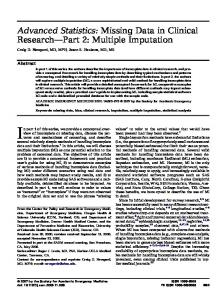
Figure 1: Histogram of number of Sexual Partners by Gender and by Survey Mode As shown in Table 1, the discrepancy between men and women is not significant for respondents interviewed under CASI questionnaires, while the discrepancy is significant for those obtained using face-to-face surveys. This also provides support for treating CASI responses as the gold standard as assumed earlier.

Table 1. Mean number of Sexual Partners by Gender and by Survey Data Sources Men (s.e.) Women (s.e.) Mean Number of SPs 15.20 (32.58) 4.74 (7.35) General Social Survey 1996 Mean Lg(Number of SPs) 1.86 (1.26) 1.17 (0.92) N 1024 1305 Mean Number of SPs 8.68 (12.37) 4.09 (4.14) Mode Experiment Mean Lg(Number of SPs) 1.49 (1.26) 1.16 (0.88) Tourangeau and Smith, 1996 N 37 65

2.4 Missing Data Pattern and Analysis Plan

10

Self-Administrated Reports

800

The validation data is comprised of the respondents interviewed under CASI in the mode experiment conducted by Tourangeau and Smith (1996). The primary survey in question is the 1996 GSS. We only selected the 1996 GSS responses in order to be consistent with the time frame of mode experiment. There are three major differences between the two survey designs. First of all, the inference population varies. The GSS is a national area probability adult sample and the sample in Tourangeau and Smith study is comprised of an area probability sample of adults in Cook County in Illinois. If there is little variation in the population composition and sexual behavior across geographic areas in the country, the assumption that both survey samples are randomization of the same population will be satisfied, otherwise, this factor may potentially complicate the imputation result in this study. The survey questions on the number of sex partner are also different. In the GSS the respondents are asked the “Number of opposite sex partners since age 18,” while in Tourangeau and Smith study the question is “Altogether, in your lifetime, how many men have you had sexual intercourse with? Remember to include men you may have had sex with only once”. Assuming that people are as equally likely to misreport their sexual behavior before age 18 as those happened after age 18, the study can still safely proceed. The last difference is the mode of data collection which makes the measurement error adjustment possible.

Counts

2.3 The GSS and Validation Data

The descriptive information about the variables measuring the number of sex partner by gender in each survey is presented in Table 1. As suggested by the histograms in Figure 1, the distribution of the number of SPs seems to follow Poisson distribution, and it is also supported by a large sample variance compared to the group means. Ttests for comparisons on means across gender are conducted based on log scales to approximate normality assumptions.

400

This article is not attempting to answer the question that which cause is more plausible. The above review provides guidance in locating potential validation data and improving survey design in the future to facilitate building imputation model which will be discussed in later sections.

Specifically, the GSS instruments were administrated using face to face interviews and the part of data selected from Tourangeau and Smith study is administrated using CASI.

0

condition (an instrument alike a lie detector) offer better consistency between the gender groups.

***

missing values in the rectangular units-by-variables data matrix to be analyzed, even if no attempt was made to record some of the missing values” (Rubin 1987). Measurement error treated as a missing data problem can be handled by an imputation method.

2821

Section on Survey Research Methods

A linkage of connecting the mis-measured and true values of this sensitive attribute is established to model measurement error. Since only the weak link is available in this study, stronger assumptions are required in order to carry out imputation. Missing at random (MAR) assumption is commonly assumed for this type of validation based study (Cole, Chu et al. 2006). This condition is satisfied when both the GSS and Tourangeau and Smith data are random samples of the same population geographically and periodically, or stratified samples with stratification on common covariates (in this study, only age, education year and marital status are shared between the two datasets). However, because no subjects are observed for both measures, MAR may be an overly strong assumption, though untestable. Thus, errorreduction performance is proposed to be assessed under not missing at random assumption. Multiple imputation techniques developed under a parametric Bayesian model are used to generate multiple

synthetic data vectors for sensitive attribute with measurement error corrected. The resulting imputed data is then appended with the original public data as the released public data. One advantage for this method over other measurement error treatments is that it offers great flexibility and simplicity for researchers to conduct statistical analysis without measurement error complications by fitting models using corrected responses. Another advantage is the bias reduction in statistical model estimation involving this sensitive attribute when compared with the estimate by using the original responses. Table 2 shows the missing data pattern. The ‘true’ attributes, i.e. CASI responses, for all subjects in GSS are missing. The ‘true’ and mis-measured responses, i.e. face to face responses, have not been jointly observed. The common variables in the two surveys are served as a bridge to build relationships between the ‘true’ and mismeasured responses.

Table 2: Missing data structure for the number of sexual partners responses CASI Responses Face- to- face Responses Shared Covariates Survey A: GSS 1996 Missing Observed Observed Survey B: Tourangeau and Smith (1996) Observed Missing Observed From the social presentation mechanism point of view, the distribution of measurement error of SPs in an adult population may reflect the mixture of people who always intentionally over-report with positive measurement error, such as men, and people who always tend to under report with negative measurement errors, such as women. Thus, I create two independent samples by gender, and within each gender group, a relative simple measurement error structure exists. The model setup follows the following steps: Step 1: Missing Mechanism Justification As many as possible covariates are included in the model to protect imputation model misspecification. Limited by data, the two surveys only share three covariates. To test the Missing Completely at Random assumption (MCAR), a propensity scoring model is fitted using logistic regression to estimate the conditional probability of assigning a particular subject to the GSS in the concatenated data (Rosenbaum and Rubin, 1983). To be concrete, an indicator variable was created which equals one if the observation comes from GSS survey and zero if otherwise. The propensity score is defined as pˆ i = log it ( Ri = 1| Z ) . pˆ i was then sorted and grouped into deciles. Within each decile, the proportion of subjects belonging to GSS data is computed. The Chi-Square test

for homogeneity χ df2 =10 = 32.60 is significant at .05 level implying the MCAR assumption is not plausible. Step 2: Model Setup Assuming the accurate values of CASI responses for the GSS sample are missing at random, the following joint likelihood of X and Y conditional on Z are proceeded: f ( X , Y | Z ,α , β ,θ ) where, Y : reports of the number of SPs from the 1996 GSS and are subject to measurement error X : reports of the number of SPs from the Tourangeau and Smith data and are treated as the gold standard Z : shared covariates, including age (years), education level (school years) and marital status (married/partnered, widowed, divorced/separated and never married). α , β : Coefficients in the mean function of X and Y θ : Covariance of X and Y on Z . Step 3: Conditional Covariance Assumption Justification Given the data contain no information about the conditional covariance of X and Y, assumptions had to be imposed to proceed the imputation. The treatment for the correlation between distinct variables from two surveys in statistical matching literature sheds some light on making assumptions. The usual default assumption of zero-

2822

Section on Survey Research Methods

conditional covariance helps reduce the complexity of model. The zero-conditional covariance assumption implies X ' s relationship to Y can be totally inferred from X ' s relationship to Z and Y ' s relationship to Z . However, in this study, X and Y are designed to measure the same underlying concept. The relationship between X and Y is captured by the measurement error which is believed to be related to variables beyond Z . Therefore, the conditional independence assumption may not be plausible in this application. To illustrate the general approach of this measurement error correction method, the current study is conducted under conditional independence assumption, that is θ = 0 . The robustness of this method should be assessed using sensitivity analysis in which θ takes several values throughout the spectrum of its data range as given by Kadane (1978). Although such analysis are not been carried out in this study, the research plan is outlined as follows. Consider the complete variance covariance matrix of X, Y and Z representing the interrelationships of the three set of variables: ⎡ V (X ) V ( X ,Y ) V ( X , Z )⎤ ⎢ ⎥ V ( X , Y , Z ) = ⎢V ′ ( X , Y ) V (Y ) V (Y , Z ) ⎥ ⎢V ′ ( X , Z ) V ′ ( Y , Z ) V ( Z ) ⎥⎦ ⎣ The specification of V ( X , Y | Z ) can be estimated through matrix addition and multiplication as −1 V ( X , Y ) = V ( X , Y | Z ) + V ′ ( Z , X )V ( Z ) V (Y , Z )

(Anderson

1958).

By

simple

algebra,

V ( X , Y | Z ) = V ( X , Y ) − V ′ ( Z , X ) V ( Z ) V (Y , Z ) −1

.

Because 0 ≤ V ( X , Y ) ≤ SD ( X ) SD (Y ) , the lower and upper bounds of conditional covariance are −1 −V ′ ( Z , X ) V ( Z ) V ( Y , Z ) and SD ( X ) SD ( Y ) − V ′ ( Z , X ) V ( Z ) V (Y , Z ) . This provides a bound on the conditional covariance of X and Y in terms of the covariance of X and Z , covariance of Y and Z , variance of X and Y , which can all be estimated using the two survey data. The analysis can be proceeded by setting θ multiple values within this interval and then create multiple imputations using Bayesian method for each θ . The sensitivity of θ on the post error correction gender discrepancy according to the internal validity check may be evaluated. The θ value that yields the smallest gender discrepancy will be used to produce the final imputes. −1

2.5 Imputation Model under Conditional Independent Assumption

Conditional independence implies θ = 0 . Then the initial Joint Likelihood can be reduced to f ( X , Y | Z , α , β , θ ) = f ( X | Z , α ) f (Y | Z , β ) . Since the function of α and β can be fully factorized, it is

sufficient to draw inference on α using f ( X | Z , α ) and

on β using f (Y | Z , β ) separately. The algorithm for making inference on α and creating imputes for accurate measures for the GSS respondents is described as below. Assume a Poisson distribution of X , then P ( X | Z , α ) ~ Pois ( λi ) and log ( λi ) = ziT a . The density

function of X given Z and α is n 1 P ( X | Z , α ) = ∏ λi exp ( −λi ) i =1 xi ! The posterior distribution of α will have the form: P (α | X , Z ) ∝ P ( X | Z , α ) P (α ) Assuming independent diffuse prior on α , the posterior distribution of α conditional on data is proportional to: n

p

i =1

k =1

(

P (α | X , Z ) ∝ ∏ Pois ( λi )∏ N k 0, σ 2

)

where p is the dimensions of α . This posterior distribution does not have a standard form. Therefore, the Markov-chain Monte-Carlo technique is applied to making inference of α . The Bayesian inference was conducted using WinBUGS. When only a single imputation is produced for each missing value, analyses of the resulting data typically treat the imputed values as if they were true values. This usually results in under estimating the standard errors. To account for the uncertainty of imputing, multiple sets of imputations, say M, are produced for the missing values. Each of the M data sets is analyzed using the same analysis method, and the M analyses are combined in a simple way to produce an inference that incorporated the proper variability (Rubin 1987). Specifically, each of the M sets of imputations for the missing values of accurate measure of the number of SPs for the GSS respondents are created via the following two steps: 1. Draw αˆ from its approximate posterior distribution pˆ (α | X , Z ) . 2. For each respondent in the GSS sample of size n , draw xˆ ~ Pois λˆ ; i = 1, 2,..., n , where λˆ = zT αˆ . i

(

( ) i

l , l = 1, 2,..., M Xˆ GSS = Xˆ GSS

use in addition to Y .

2823

i

)

i

will be released for public

Section on Survey Research Methods

In response to the confidentiality concern, Y is perturbed in a similar fashion and Yˆ = Yˆ l , l = 1, 2,..., M is

Convergence statistics. All the plots and statistics not shown here suggest convergence is achieved.

generated and is released to public in place of Y .

After corrected for measurement error, the imputed mean number of SPs for men is 12.65, compared with 15.2 for interviewer administrated reports. The imputed mean of SP for women equals 4.014 compared with 4.74 for interviewers’ administrated reports. The corrected discrepancy between men and women (8.64) is smaller than the original discrepancy (10.46). The data quality is modestly improved. However, the non-significant discrepancy in Tourangeau and Smith data was not duplicated in the imputed GSS data. There are several potential reasons. The independent assumption between X and Y conditional on Z may be not plausible. Rubin (1987) states that “within the multiple-imputation framework it is not necessary to assume conditional independence or any other specific choice for the parameters of conditional association, because each set of imputations can be made for a different choice of parameters of conditional association.” Further sensitivity analysis under conditional dependent assumptions may provide more evidence for bias reduction. Another possible reason is the basic demographic characteristics can not fully explain the measurement error due to social desirability. Other potential predictors such as occupations, job characteristics, living pattern, financial situations, religions etc. may help improve the model. Similar type of analysis should be conducted when more suitable data are available.

(

GSS

)

GSS

2.6 Imputation Model under Conditional Dependence Assumption Under the conditional dependent assumption and set θ to a value within the possible range of conditional covariance of X and Y as derived earlier. To illustrate the algorithm, let θ = r1 then the joint likelihood takes this form f ( X , Y | Z , α , β , r1 ) ~ BP ( λ1i , λ2 i , λ3i ) where

log ( λ1i ) = zit α ;log ( λ2i ) = zit β ; log ( λ3i ) = zit r1 . The joint distribution can be written as P ( X , Y | Z , α , β , r1 ) =

∑ n

i =1

⎛ exp ⎜ ⎝

∑ ( −λ ) 3

ki

k =1

⎞ λ1ii ⎟ ⎠ xi ! x

λ2yi

i

yi !

(

∑

min xi , yi i=0

) x y ⎛ λ3i ⎞ ⎛ ⎞⎛ ⎞ ⎜ ⎟⎜ ⎝ i ⎠⎝

⎟ i !⎜ ⎝

i⎠

λ1i λ2i

⎟ ⎠

Assuming independent diffuse prior on (α , β ) , Bayesian inference can be made using MCMC approach and Dˆ = Xˆ l , Yˆ l ; l = 1, 2,..., M are created by random GSS

((

GSS

GSS

)

)

draws from the approximate posterior predictive joint distribution. 2.7 Evaluation Methods for Measurement Error Correction and Confidentiality Protection Two sets of evaluations will be developed to address the two research goals respectively. The evaluation method for measurement error correction performance can be carried out by comparing the means in imputed number of SPs between men and women. Smaller discrepancies suggest better bias reduction. As statistically perturbations have been applied to the original sensitive responses in GSS data to protect confidentiality, the information loss is expected from statistical estimations using the perturbed data. The potential statistical information loss will be evaluated by comparing point estimates and interval estimates using perturbed data with those using original responses. Large information loss suggests poor fit of imputation models and/or improper model assumptions. 3. Results Imputations are constructed under the assumption of conditional independence assumption. Separate Poisson imputation models were fit for men and women. The thinning interval used in the simulation was 10, with 1000 posterior samples. Diagnostics for convergence were conducted by examining the autocorrelation plots, trace plots, density plots, as well as Gelman-Rubin

4. Discussions and Practical Implications Based on the results, this method has shown to be effective in reducing measurement error and easy to implement. The bias reduction performance is very promising, and the inflated disclosure harm due to releasing corrected data to the public is also easily controlled. This methodology also provides a platform for suggestions to improve future survey design with the goal of reducing Total Survey Error. Studies have shown that topic sensitivity increases respondents’ perception of disclosure risk and harm especially when confidentiality is not fully assured. Hence impairing survey participation (Singer, Couper, and Mathiowetz, 1993; Singer, Van Hoewyk, and Neugebauer, 2003; Hillygus, Nie, Prewitt, and Pals, 2006) and biasing the statistical estimation because of survey nonresponse (Groves et al, 2002). Assurances of confidentiality by promise of randomized responses improve sensitive responses in terms of both response rates and response quality (Singer, Hippler, and Schwarz, 1992; Singer, Von Thurn, and Miller, 1995). With this post-survey adjustment perspective in mind,

2824

Section on Survey Research Methods

survey requests can be properly altered by offering better confidential assurance by promising to release only randomized responses in order to strengthen trust between researchers and respondents, hence improving both response rate and response quality for sensitive topics. Furthermore, the robustness of the imputation model can be enhanced by accurate information about sensitive response quality and richer covariates, which are related to both sensitive attributes and social presentation propensity (Rubin, 1987). The bridge between social desirable reports and ‘true’ values for the sensitive attributes can be easily built by implementing concurrent randomized experiment where a random sub-sample is assigned to a survey condition assumed to produce error free responses (for example, self administrated mode of data collection or bogus pipeline instrument to remove social presentation effects for the set of sensitive questions). Responses for the remaining questionnaire can be readily obtained by resuming the original survey condition to avoid potential mode effect in measurements, and the scope of selecting covariates for the imputation model is expanded as well. Cautions should be taken in designing questionnaire to avoid differential context or order effects (Tourangeau, Rips and Rasinski, 2000). Acknowledgements I thank Roger Tourangeau for making this study possible by sharing his data. I also thank Norman Brown, Robert Groves, Partha Lahiri and Trivellore Raghuanathan for suggestions and advices. References Alexander, M. G. and T. D. Fisher (2003). "Truth and consequences: Using the bogus pipeline to examine sex differences in self-reported sexuality." Journal of Sex Research 40(1): 27-35. Biemer, P. (1991). Measurement errors in surveys. New York, Wiley. Brewer, D. D., J. J. Potterat, et al. (2000). "Prostitution and the sex discrepancy in reported number of sexual partners." Proceedings of the National Academy of Sciences of the United States of America 97(22): 12385-12388. Brewer, D. D., J. J. Potterat, et al. (2005). "Randomized trial of supplementary interviewing techniques to enhance recall of sexual partners in contact interviews." Sexually Transmitted Diseases 32(3): 189-193. Brown, N. R. (1995). "Estimation strategies and the judgment of event frequency." Journal of Experimental Psychology: Learning, Memory, and Cognition 21(6): 1539-1553.

Brown, N. R., P. Sedlmeier, et al. (2002). Encoding, representing, and estimating event frequencies: A multiple strategy perspective. New York, NY, US, Oxford University Press. Brown, N. R. and R. C. Sinclair (1999). "Estimating number of lifetime sexual partners: Men and women do it differently." Journal of Sex Research 36(3): 292-297. Cole, S. R., H. Chu, et al. (2006). "Multiple-imputation for measurement -error correction." International Journal of Epidemiology 35: 1074-1081. Crawford, M. and D. Popp (2003). "Sexual double standards: A review and methodological critique of two decades of research." Journal of Sex Research 40(1): 13-26. Fuller, W. A. (1987). Measurement Error Models. New York, John Wiley & Sons Inc. Groves, R. M. (2002). Survey nonresponse. New York, Wiley. Karlis, D. and I. Ntzoufras (2005). "Bivariate Poisson and diagonal inflated bivariate Poisson regression models in R." Journal of Statistical Software 14(10). Lambert, D. (1993). "Measures of Disclosure Risk and Harm." Journal of Official Statistics 9(2): 313-331. Morris, C. and F. Scheuren (2001). "Statsitical Matching: A Paradigam for Assessing the Uncertainty in the Procedure." Journal of Official Statistics 17(3): 407322. Morris, M. (1993). "Telling Tails Explain the Discrepancy in Sexual Partner Reports." Nature 365(6445): 437-440. Rodger, W. L. (1984). "An Evaluation of Statsitical Matching." Journal of Business and Economic Statistics 2(1). Rubin, D. (1987). Multiple Imputation for Nonresponse in Surveys. New York, Wiley & Sons. Singer, E., N. A. Mathiowetz, et al. (1993). "The Impact of Privacy and Confidentiality Concerns on Survey Participation - the Case of the 1990 United-States Census." Public Opinion Quarterly 57(4): 465-482. Singer, E., D. R. Vonthurn, et al. (1995). "Confidentiality Assurances and Response - a Quantitative Review of the Experimental Literature." Public Opinion Quarterly 59(1): 66-77. Tourangeau, R., L. J. Rips, et al. (2000). The Psychology of Survey Response. Cambridge, Cambridge University Press. Tourangeau, R. and T. W. Smith (1996). "Asking sensitive questions - The impact of data collection mode, question format, and question context." Public Opinion Quarterly 60(2): 275-304. Wiederman, M. W. (1997). "The truth must be in here somewhere: Examining the gender discrepancy in self-reported lifetime number of sex partners." Journal of Sex Research 34(4): 375-386.

2825