tural Engineer, James H. Everitt, Range Scientist, and Joe M. Bradford, .... Pathfinder Pro XRS system (Trimble Navigation Limited, ...... Escobar, D. E., J. H. Everitt, J. R. Noriega, M. R. Davis, and I. Ca- vazos ... R. L. Travis, and R. B. Hutmacher.
USING MULTISPECTRAL IMAGERY AND LINEAR SPECTRAL UNMIXING TECHNIQUES FOR ESTIMATING CROP YIELD VARIABILITY C. Yang, J. H. Everitt, J. M. Bradford ABSTRACT. Vegetation indices derived from multispectral imagery are commonly used to extract crop growth and yield information. Spectral unmixing techniques provide an alternative approach to quantifying crop canopy abundance within each image pixel and have the potential for mapping crop yield variability. The objective of this study was to apply linear spectral unmixing techniques to airborne multispectral imagery for estimating grain sorghum yield variability. Five time-sequential airborne multispectral images and yield monitor data collected from a grain sorghum field were used for this study. Both unconstrained and constrained linear spectral unmixing models were applied to the images to generate crop plant and soil abundances for each image and for all 26 multi-image combinations of the five images. Yield was related to unconstrained and constrained plant and soil abundances as well as to the normalized difference vegetation index (NDVI) and the green NDVI (GNDVI). Results showed that unconstrained plant abundance had better correlations with yield than NDVI for all five images, but GNDVI had better correlations with yield for the first three images. Unconstrained plant abundance derived from the fourth image provided the best overall correlation with yield (r = 0.88). Moreover, multi-image combinations generally improved the correlations with yield over single images, and the best three-image combination resulted in the highest overall correlation (r = 0.90) between yield and unconstrained plant abundance. These results indicate that linear spectral unmixing techniques can be a useful tool for quantifying crop canopy abundance and mapping crop yield. Keywords. Abundance, Endmember, Linear spectral unmixing, Multispectral imagery, Vegetation index, Yield monitor, Yield variability.
R
emote sensing data, including ground reflectance spectra, satellite imagery, and airborne imagery, have long been used to extract crop growth and yield information. Although these data can be directly related to crop biophysical parameters, vegetation indices derived from various wavebands in the data are more effective and therefore are more widely used. Many of these indices are formed from combinations of red and nearinfrared (NIR) wavebands. Indices based on these two bands exploit the fact that living green vegetation absorbs radiation in the red band, due to the presence of chlorophyll and other absorbing pigments in leaves, and strongly reflects radiation in the NIR band, because of the internal structure of the leaf that is responsible for the high reflection. Two of the earliest and most widely used vegetation indices are the simple ratio (NIR/Red) (Jordan, 1969) and the normalized difference vegetation index [NDVI = (NIR − Red)/(NIR + Red)] (Rouse et al., 1973). These indices along with other vegetation indices
Submitted for review in November 2005 as manuscript number IET 6192; approved for publication by the Information & Electrical Technologies Division of ASABE in December 2006. Presented at the 2005 ASAE Annual Meeting as Paper No. 051018. Mention of trade names or commercial products in this article is solely for the purpose of providing specific information and does not imply recommendation or endorsement by the USDA. The authors are Chenghai Yang, ASABE Member Engineer, Agricultural Engineer, James H. Everitt, Range Scientist, and Joe M. Bradford, Supervisory Soil Scientist, USDA-ARS Kika de la Garza Subtropical Agricultural Research Center, Weslaco, Texas. Corresponding author: Chenghai Yang, USDA-ARS Kika de la Garza Subtropical Agricultural Research Center, 2413 E. Highway 83, Weslaco, TX 78596; phone: 956-969-4824; fax: 956-969-4893; e-mail: cyang@ weslaco.ars.usda.gov.
derived from the visible to NIR portion of the spectrum are often used to quantify crop variables such as leaf area index, biomass, and yield (Tucker et al., 1980; Wiegand et al., 1991; Thenkabail et al., 1995; Yang and Anderson, 1999; Plant et al., 2000; Yang et al., 2001). Yang et al. (2000) and Yang and Everitt (2002) used two band ratios (NIR/Red and NIR/ Green), NDVI, and the green NDVI [GNDVI = (NIR − Green)/(NIR + Green)] derived from airborne color-infrared (CIR) imagery to generate yield maps for delineating withinfield spatial variability as compared with yield monitor data. Although vegetation indices are by far the most popular techniques for extracting quantitative biophysical information, many, if not most, indices only use two spectral bands in the data. This may be sufficient if the data contain only a few bands. However, if a large number of bands are available, as in some multispectral and hyperspectral data, other techniques that can use all the bands in the data may have the potential to offer better results. Linear spectral unmixing is one such technique (Adams et al., 1986). Spectral mixing occurs when materials with different spectral properties are represented by a single image pixel. Multispectral and hyperspectral imagery can be viewed as a collection of band images, and each image pixel contains a spectrum of reflectance values for all the wavebands in the imagery. These spectra may be considered as the signatures of ground materials such as crop plants or soil, provided that the material occupies the whole pixel. Spectra of mixtures can be analyzed with linear spectral unmixing, which models each spectrum as a linear combination of a finite number of pure spectra of the materials located in the pixel area, weighted by their fractional abundances (Adams et al., 1986; Smith et al., 1990). The unique ground materials are referred to as endmembers, and
Transactions of the ASABE Vol. 50(2): 667−674
2007 American Society of Agricultural and Biological Engineers ISSN 0001−2351
667
their spectra are referred to as endmember spectra. A simple linear spectral unmixing model has the following form: yi =
m
∑ aij x j + ε i , i = 1, 2, ..., n
j =1
(1)
where yi = measured reflectance in band i for a pixel aij = known or measured reflectance in band i for endmember j xj = unknown fractional abundance for endmember j ei = residual between measured and modeled reflectance for band i m = number of endmembers n = number of spectral bands. This model is referred to as the unconstrained linear spectral unmixing model. For constrained linear spectral unmixing, the following additional condition should be satisfied: m
∑ xj =1
j =1
(2)
That is, the fractional abundances for all the endmembers should sum to unity. Nevertheless, both unconstrained and constrained unmixing can result in negative abundance values and values greater than 1 for any endmember. Assuming that the endmembers are not linearly dependent, the mixing fractions can be determined from the data. For a given number of spectral bands n, an exact solution can be found for each pixel for the unconstrained model if m = n and for the constrained model if m = n + 1. However, if m < n for unconstrained unmixing or if m < n + 1 for constrained unmixing, then a least squares fitting procedure can be applied to obtain the best fit. The fractional abundances determined by linear spectral unmixing may be preferred to band ratios and NDVI for tracking spectrally defined materials (i.e., endmembers) since it uses all the bands in the data (Bateson and Curtiss, 1996). When linear spectral unmixing is applied to an image, it produces a suite of abundance images, one for each endmember in the model. Like a NDVI image, each abundance image shows the spatial distribution of the spectrally defined material. Different varieties of linear spectral unmixing have been used with multispectral and hyperspectral imagery for mapping the abundance and distributions of geological materials and vegetation types in many different applications (Adams et al., 1986, 1995; Roberts, et al., 1998; Lobell and Asner, 2004). However, there has been no report on the use of this technique for estimating crop yield variations. As many vegetation indices such as NDVI are an indirect measure of plant vigor and abundance, the fractional abundance of crop plants determined from linear spectral unmixing is a more direct measure of plant abundance and provides a more intuitive link between image data and ground observations. For example, field observers can readily understand the significance of a pixel having 80% green vegetation and 20% soil, but they have more difficulty interpreting the equivalent band reflectance values and vegetation index values. The objectives of this study were to: (1) apply linear spectral unmixing techniques to airborne CIR imagery for estimating grain sorghum plant and soil abundances, and
668
(2) relate grain yield to plant and soil abundances as well as to NDVI and GNDVI.
METHODS
IMAGERY AND YIELD DATA PREPROCESSING Airborne digital CIR images and yield monitor data collected from a 21 ha grain sorghum field in south Texas in 1998 were used for this study. The geographic coordinates near the center of the field were 26° 29′ 27″ and 98° 00′ 03″ W. Grain sorghum (Asgrow 570) was planted to the field on 15 February and was harvested on 22 June. The CIR imagery was acquired on five different dates during the growing season using a three-camera digital imaging system described by Escobar et al. (1997). The system consisted of three Kodak MegaPlus charge-coupled device (CCD) digital cameras and a computer equipped with three image-grabbing boards. The cameras were filtered for spectral observations in the visible green (555-565 nm), red (625-635 nm), and NIR (845- 857 nm) bands. The image-grabbing boards had the capability to capture 8-bit image frames with 1024 × 1024 pixels. CIR images were obtained at an altitude of approximately 1680 m (5500 ft) between 12:00 and 15:00 h local time under sunny conditions on five dates: 15 and 22 April, 18 and 29 May, and 16 June 1998. A Cessna 206 aircraft was used to acquire the imagery. The imagery had a ground pixel size of approximately 1 m. The three band images in each composite CIR image were first registered to correct the misalignments among them. The registered CIR images were then rectified to the Universal Transverse Mercator (UTM), World Geodetic Survey 1984 (WGS-84), Zone 14, coordinate system based on ground control points located with a submeter-accuracy GPS Pathfinder Pro XRS system (Trimble Navigation Limited, Sunnyvale, Cal.). All rectified images were resampled to a spatial resolution of 1 m using the nearest-neighbor resampling method. Total RMS (root mean square) errors for all rectified images were less than 2 m. For radiometric calibration, reflectance spectra were taken from three sites (an asphalt road, a concrete parking lot, and a roof) within the image. These sites had stable reflectance response over the season and represented a wide range of reflectance values. The reflectance spectra for the three sites were measured using a FieldSpec HandHeld spectroradiometer (Analytical Spectral Devices, Inc., Boulder, Colo.) sensitive in the 350 to 1050 nm portion of the spectrum with a nominal spectral resolution of 1.4 nm. Each rectified multispectral image was converted to reflectance based on the calibration equations for the three bands determined between the measured reflectance and the digital count values extracted from the image at the three sites. The procedures for image registration, rectification, and calibration were performed using ERDAS IMAGINE (Leica Geosystems Geospatial Imaging, LLC, Norcross, Ga.). The images were then used in ENVI (Research Systems, Inc., Boulder, Colo.) for linear spectral unmixing analysis. Yield data were collected using an AgLeader Yield Monitor 2000 system (Ag Leader Technology, Ames, Iowa) integrated with a submeter AgGPS 132 receiver (Trimble Navigation Limited, Sunnyvale, Cal.). Instantaneous yield, moisture, and GPS data were simultaneously recorded at 1 s intervals. The combine equipped with the yield monitoring
TRANSACTIONS OF THE ASABE
system had an effective cutting width of 8.69 m (nine 38 in. rows). The yield monitor was calibrated to ensure data accuracy before grain was harvested in late June. The yield and GPS data were viewed and evaluated using SMS Basic software (Ag Leader Technology, Ames, Iowa). Points falling on the top of a harvested path or points with extreme high or low values along each path were first examined and then removed if they were determined to be erroneous. The filtered yield data were exported in ASCII format for further filtering and processing using self-developed programs. An optimum time lag of 12 s, as determined using the method of Yang et al. (2002), was used to align yield data with position data. Yield data were adjusted to 14% moisture content. LINEAR SPECTRAL UNMIXING ANALYSIS The first important step in linear spectral unmixing analysis is to determine the endmembers and their spectra. Many studies of spectral unmixing have used uncalibrated spectra derived from training areas of images as endmember spectra (Adams et al., 1995). When relatively pure, image endmembers can be used to model mixed pixels within an image. Because of different plant growth stages and temporally variant soil surface and moisture conditions during a growing season, the reflectance spectra of crop plants and soil background change from time to time. Therefore, endmember spectra derived from an image should be used only for that particular image, no matter whether the image is radiometrically calibrated or not. It is not feasible to use image endmember spectra derived from one image taken on a particular date for images taken on other dates. In this study, grain sorghum plants and bare soil were selected as two meaningful endmembers. To obtain pure spectra for sorghum plants, 20 pixels that had a bright red color (corresponding to healthy plants on a CIR image) were first identified from the 15 April image, and the same pixels were then viewed on the other four images to make sure the training pixels on all five images represented some of the most healthy sorghum plants. Similarly, 20 pixels that contained pure bare soil were identified from the first image and verified on the other four images. The endmember spectra for plants and soil for each image were obtained by averaging the spectra of the respective training pixels from that image. Although the same training pixel locations were used to extract endmember spectra from all the images in this study, different training pixels could have been used for different images as long as reliable pixels were identified from each image. Alternatively, computerized methods such as the pixel purity index and the ndimensional visualizer in ENVI can be used to identify purest pixels for the endmembers. However, these automatic methods are not always reliable. For example, weed plants can be mixed with crop plants, and atypical soil surface areas with too dark or too bright colors can be misidentified as typical soil. Since there were only two endmembers in this particular application, simple manual identification of pure pixels of each endmember was reliable and efficient. Originally, there were five CIR images, and each had three bands. By stacking two to five of the CIR images, 26 new images with 6 to 15 bands were generated. Both unconstrained and constrained linear spectral models were applied to: (1) the five individual CIR images, (2) the ten combinations of any two CIR images, (3) the ten combinations of any three CIR images, (4) the five combinations of any four CIR images, and (5) the combined image from the five CIR images.
Vol. 50(2): 667−674
Since the number of endmembers (m = 2) was smaller than the number of bands in each original CIR image (n = 3) or in each combined image (n = 6, 9, 12, or 15), the least squares fitting procedure was used to determine the fractional abundance images for both unconstrained and constrained unmixing models. In order to examine how variations in endmember spectra affect the results, 27 different plant spectra were generated by varying the spectrum values for each of the three bands at three different levels. The digital spectrum values for each band were set to be 0.8, 1.0, or 1.2 times the original plant spectrum values. Both unconstrained and constrained spectral unmixing procedures were performed on the 29 May image for each of the 27 plant spectra. GIS AND STATISTICAL ANALYSIS The CIR images and fractional abundance images were converted into grids in ArcInfo (ESRI, Inc., Redlands, Cal.). The preprocessed yield data were imported into ArcInfo as a point coverage. Since the combine’s effective cutting width was 8.69 m and the cell size of the image data was 1 m, these images were aggregated by a factor of 9 to increase the cell size to 9 m. The digital value for each output cell for each band image and each fractional abundance image was the mean of the 81 input cells that the 9 × 9 m output cell encompassed. The yield value for each output cell was the mean of the yield points falling within the 9 × 9 m output cell. On the average, each output cell contained seven yield points. In order to see how the aggregation of abundance values from 1 m cell size to 9 m cell size was compared with the abundance values derived directly from images with 9 m cell size, the five images were aggregated from 1 m cell size to 9 m cell size. Then both unconstrained and constrained linear spectral unmixing models were applied to the images with 9 m cell size. Vegetation indices NDVI and GNDVI were derived from the three spectral bands of each CIR image for comparison with spectra unmixing results. Correlation matrices were calculated among grain sorghum yield, the two vegetation indices, and all the plant and soil abundance images. Linear regression was performed to determine the best-fitting equations and their coefficients of determination (r2) for relating yield to each vegetation index and to each fractional abundance index. Statistical analysis was performed using SAS software (SAS Institute Inc., Cary, N.C.).
RESULTS AND DISCUSSION
Table 1 summarizes the simple statistics of plant and soil abundances derived from the five time-sequential airborne CIR images for the grain sorghum field based on both the unconstrained and constrained unmixing models. The statistics for the sum of plant and soil abundances are also presented. Ideally, fractional abundance values should be within the 0-1 range, but in practice abundances may assume negative values and values greater than 1. This is because spectral unmixing results can be affected by the purity of the endmembers and the completeness of endmembers. Moreover, the linearity assumption of linear spectral unmixing is at best an approximation of the generally non-linear mixing of surface materials. Therefore, the simple statistics of the abundance values can be used to determine how well the linear
669
Table 1. Simple statistics of endmember abundances derived from airborne color-infrared images obtained from a 21 ha grain sorghum field in south Texas on five different dates in 1998. Endmember Abundance[b] Statistic[a] 15 April 1
UPA
USA
UPA +USA
CPA
CSA
CPA +CSA
0.0% −0.02 0.56 0.19 1.19 0.9%
1.5% −0.10 0.33 0.17 0.92 0.0%
0.0% 0.69 0.89 0.07 1.11 7.5%
1.0% −0.22 0.46 0.23 1.29 1.2%
1.2% −0.29 0.54 0.23 1.22 1.0%
0.0% 1.00 1.00 0.00 1.00 0.0%
22 April 1
0.0% −0.04 0.63 0.26 1.34 5.2%
12.3% −0.21 0.25 0.22 0.94 0.0%
0.0% 0.56 0.88 0.10 1.18 11.7%
0.1% −0.06 0.62 0.27 1.36 5.0%
5.0% −0.36 0.38 0.27 1.06 0.1%
0.0% 1.00 1.00 0.00 1.00 0.0%
18 May 1
0.0% 0.04 0.86 0.18 1.17 17.9%
14.8% −0.07 0.11 0.14 0.89 0.0%
0.0% 0.77 0.97 0.05 1.12 26.9%
0.2% −0.05 0.83 0.22 1.27 20.0%
20.0% −0.27 0.17 0.22 1.05 0.2%
0.0% 1.00 1.00 0.00 1.00 0.0%
29 May 1
0.0% 0.10 0.80 0.21 1.12 7.6%
16.6% −0.12 0.16 0.19 0.86 0.0%
0.0% 0.75 0.96 0.07 1.15 30.0%
0.2% −0.08 0.76 0.25 1.20 14.6%
14.6% −0.20 0.24 0.25 1.08 0.2%
0.0% 1.00 1.00 0.00 1.00 0.0%
16 June 1
0.0% 0.10 0.73 0.24 1.16 7.2%
10.8% −0.12 0.23 0.22 0.92 0.0%
0.0% 0.81 0.96 0.04 1.09 16.5%
0.4% −0.05 0.69 0.26 1.19 5.8%
5.8% −0.19 0.31 0.26 1.05 0.4%
0.0% 1.00 1.00 0.00 1.00 0.0%
[a]
1 = samples with abundance values greater than 1 as a percentage of the total number of samples. [b] UPA = unconstrained plant abundance, USA = unconstrained soil abundance, CPA = constrained plant abundance, and CSA = constrained soil abundance.
unmixing models work for a particular image. Table 1 also presents the percentage of samples that had negative values and the percentage of samples that had values greater than 1. Overall, the majority of the abundance values for the two endmembers fell in the 0-1 range for the five time-sequential images based on the unconstrained and constrained models. The 15 April image had the best results for the unconstrained model, with only 0.9% of the plant abundance values greater than 1 and 1.5% of the soil abundance values less than 0. This image also had the best results for the constrained model, with 1.2% of the plant abundance values greater than 1 and 1.2% of the constrained soil abundance values less than 0. The other four images had larger percentages of abundance values falling outside the 0-1 range. For the unconstrained model, the 18 May image had the largest percentage of plant
670
abundance values greater than 1 (17.9%), while the 29 May image resulted in the largest percentage of soil abundance values less than 0 (16.6%). For the constrained model, the 18 May image had the largest percentage of plant abundance values greater than 1 (20.0%) and the largest percentage of soil abundance values less than 0 (20.0%). Mean unconstrained plant abundance was the lowest (0.56) on 15 April, increased to 0.63 on 22 April, reached its maximum (0.86) on 18 May, and then decreased to 0.80 on 29 May and 0.73 on 16 June. This general trend agreed with the plant growth pattern of grain sorghum. The 15 April image was taken when plants were at the boot stage (plant head extended into the flag leaf sheath) and canopy cover was over 50%, and the 22 April image was taken one week later while the plants were predominately in the same stage. By 18 May, the plants were at the bloom stage and most of the plants were fully expanded and reached their maximum canopy cover and vigor. When the 29 May image was taken, the plants were at the soft-dough and hard-dough stages and still provided maximum canopy cover, but some of the leaves started showing dull green coloration and necrotic lesion. Although the amount of plant materials did not decrease, the plant abundance values decreased. This is because only two endmembers (plants and soil) were used in the model and the spectral deviation from the spectrum for healthy plants would lower the plant abundance estimate. The 16 June image was taken shortly before harvest, when the plants were approaching physiological maturity and the leaves were senescing. Again, although there was little change in the amount of plant materials, the spectral characteristics of the plants changed significantly, resulting in lower plant abundance estimates. As expected, mean unconstrained soil abundance had the opposite trend, with the highest value (0.33) for the 15 April image and the lowest value (0.11) for the 18 May image. The mean sums of unconstrained plant and soil abundances were 0.89, 0.88, 0.97, 0.96, and 0.96 for the five time-sequential images from 15 April to 16 June, respectively. Although the unconstrained model did not force the endmember abundances to sum to 1, these sum abundance values were close to 1, especially for the three later dates, indicating that the unconstrained two-endmember linear unmixing model was appropriate for characterizing plant and soil abundances in the images. The difference between 1 and the sum abundance value was partly due to endmembers unaccounted for (i.e., shading) in the model. For example, the unconstrained model explained only 88% of the materials for the 22 April image. In addition to shade, the wet soil background in a small portion of the field, which was being irrigated at the time of imaging, was not accounted for in the unconstrained model. For the constrained model, the sum abundance was 1 because the constrained model forced the endmember abundances to sum to 1. Therefore, endmember abundances may have been under- or overestimated if some significant endmembers were not included in the model. In fact, mean constrained plant abundance values were 0.46, 0.62, 0.83, 0.76, and 0.69 for the five time-sequential images from 15 April to 16 June, respectively. These constrained plant abundance values had a similar trend as the unconstrained values, but were consistently lower than the respective unconstrained abundance values. On the other hand, the constrained soil abundance values were consistently higher than the respective unconstrained abundance values. Therefore, unconstrained linear unmixing may be more appropri−
TRANSACTIONS OF THE ASABE
Table 2. Correlation coefficients (r) between yield monitor data and spectral variables (two vegetation indices and four endmember abundances) derived from airborne color-infrared images obtained from a 21 ha grain sorghum field in south Texas on five different dates in 1998. The spectral variables were based on the vegetation indices and abundance images aggregated from 1 m cell size to 9 m cell size. Date[b] Spectral
Variable[a] NDVI GNDVI UPA USA CPA CSA
15 April
22 April
18 May
29 May
16 June
0.709* 0.757* 0.732* −0.680* 0.696* −0.696*
0.747* 0.799* 0.788* −0.715* 0.789* −0.789*
0.775* 0.843* 0.816* −0.820* 0.797* −0.797*
0.849* 0.858* 0.877* −0.840* 0.823* −0.823*
0.837* 0.844* 0.853* −0.825* 0.858* −0.858*
[a]
NDVI = (NIR − Red) / (NIR + Red), GNDVI = (NIR − Green) / (NIR + Green). UPA = unconstrained plant abundance, USA = unconstrained soil abundance, CPA = constrained plant abundance, and CSA = constrained soil abundance. [b] * = significant at the 0.0001 level. Number of samples = 2497. Table 3. Correlation coefficients (r) between yield monitor data and spectral variables (two vegetation indices and four endmember abundances) derived from airborne color-infrared images obtained from a 21 ha grain sorghum field in south Texas on five different dates in 1998. The spectral variables were based on the vegetation indices and abundance images with 9 m cell size. Date[b] Spectral
Variable[a] NDVI GNDVI UPA USA CPA CSA
15 April
22 April
18 May
29 May
16 June
0.715* 0.762* 0.740* −0.685* 0.704* −0.704*
0.752* 0.803* 0.793* −0.719* 0.793* −0.793*
0.771* 0.845* 0.816* −0.821* 0.797* −0.797*
0.852* 0.860* 0.880* −0.842* 0.827* −0.827*
0.838* 0.845* 0.854* −0.826* 0.860* −0.860*
Table 4. Correlation coefficients (r) between yield monitor data and endmember abundances derived from different combinations of five time-sequential airborne color-infrared images obtained from a 21 ha grain sorghum field in south Texas in 1998. Endmember Abundance[b] Image
Combination[a] 1-2 1-3 1-4 1-5 2-3 2-4 2-5 3-4 3-5 4-5 1-2-3 1-2-4 1-2-5 1-3-4 1-3-5 1-4-5 2-3-4 2-3-5 2-4-5 3-4-5 1-2-3-4 1-2-3-5 1-2-4-5 1-3-4-5 2-3-4-5 1-2-3-4-5
UPA
USA
CPA
CSA
0.786* 0.833* 0.888* 0.875* 0.837* 0.887* 0.881* 0.842* 0.844* 0.881* 0.847* 0.876* 0.866* 0.860* 0.862* 0.898* 0.865* 0.865* 0.902* 0.860* 0.871* 0.871* 0.897* 0.874* 0.879* 0.884*
−0.711* −0.781* −0.846* −0.850* −0.725* −0.810* −0.817* −0.798* −0.831* −0.859* −0.742* −0.803* −0.806* −0.804* −0.830* −0.872* −0.772* −0.794* −0.849* −0.828* −0.781* −0.797* −0.843* −0.835* −0.814* −0.816*
0.779* 0.827* 0.837* 0.851* 0.850* 0.872* 0.881* 0.837* 0.839* 0.855* 0.852* 0.854* 0.856* 0.851* 0.855* 0.865* 0.868* 0.871* 0.887* 0.854* 0.868* 0.871* 0.876* 0.864* 0.878* 0.878*
−0.779* −0.827* −0.837* −0.851* −0.850* −0.872* −0.881* −0.837* −0.839* −0.855* −0.852* −0.854* −0.856* −0.851* −0.855* −0.865* −0.868* −0.871* −0.887* −0.854* −0.868* −0.871* −0.876* −0.864* −0.878* −0.878*
[a]
[a] [b]
ate than constrained linear unmixing for this particular application. Tables 2 and 3 summarize the correlation coefficients of grain yield with two vegetation indices and four plant and soil abundances for the five time-sequential airborne CIR images of the grain sorghum field based on aggregated abundance values from the abundance images with 1 m cell size and nonaggregated abundance values with 9 m cell size, respectively. A comparison of the two tables shows that the r-values based on the aggregated abundance values are essentially the same as those based on the non-aggregated abundance values. Moreover, the mean and standard deviation for the plant and soil abundances based on the non-aggregated abundance values with 9 m cell size (not shown) were exactly the same (to the 1/100) as those shown in table 1. Therefore, aggregating abundance values from 1 m cell size to 9 m cell size was a feasible approach in the correlation analysis. Grain yield was positively related to the two vegetation indices and the unconstrained and constrained plant abundances, and negatively related to the unconstrained and constrained soil abundances. GNDVI provided the best correlations with yield for the first three images, while unconstrained plant abundance had the best correlation for the 29 May image and constrained plant or soil abundance had the best correlation for the 16 June image. The unconstrained
plant abundance for the 29 May image also provided the best overall correlation with yield (0.88) among all the images. Moreover, unconstrained plant abundance had better correlations with yield than NDVI for all five images. It also gave better correlations than unconstrained soil abundance for all the images except for the 18 May image. Both constrained plant and soil abundances had identical absolute correlations with yield. However, constrained abundances had lower correlations with yield than unconstrained plant abundances for three of the five images. Table 4 presents the correlation coefficients between yield monitor data and endmember abundances derived from different combinations of the five time-sequential images. Similar to the results for the individual images, unconstrained plant abundance was generally better related with yield than unconstrained soil abundance or constrained abundances. The correlation coefficients for the best two-, three-, four-, and five-image combinations were 0.89, 0.90, 0.90, and 0.88, respectively. These r-values were slightly higher than or similar to the best r-value (0.88) for the 29 May image. Moreover, the four- and five-image combinations did not have better r-values than the three-image combination. A possible explanation for this may be that variations in the additional images were already contained in the best three-image combination and some of these additional variations might not be due to the variation in yield. Nevertheless, the unmix−
NDVI = (NIR − Red) / (NIR + Red), GNDVI = (NIR − Green) / (NIR + Green), UPA = unconstrained plant abundance, USA = unconstrained soil abundance, CPA = constrained plant abundance, and CSA = constrained soil abundance. [b] * = significant at the 0.0001 level. Number of samples = 2497.
Vol. 50(2): 667−674
1 = 15 April, 2 = 22 April, 3 = 18 May, 4 = 29 May, and 5 = 16 June. * = significant at the 0.0001 level. Number of samples = 2497. UPA = unconstrained plant abundance, USA = unconstrained soil abundance, CPA = constrained plant abundance, and CSA = constrained soil abundance.
671
Table 5. Correlation coefficients (r) between yield monitor data and endmember abundances based on 27 different plant spectra and one soil spectrum. The endmember abundances were derived from an airborne color-infrared image obtained from a 21 ha grain sorghum field in south Texas on 29 May 1998. Endmember Abundance[b] Plant Spectrum[a] 0.8-0.8-0.8 0.8-0.8-1.0 0.8-0.8-1.2 0.8-1.0-0.8 0.8-1.0-1.0 0.8-1.0-1.2 0.8-1.2-0.8 0.8-1.2-1.0 0.8-1.2-1.2
UPA
USA
CPA
CSA
0.877* 0.876* 0.875* 0.878* 0.876* 0.875* 0.878* 0.877* 0.876*
−0.840* −0.846* −0.848* −0.851* −0.856* −0.859* −0.858* −0.864* −0.866*
0.878* 0.877* 0.875* 0.879* 0.876* 0.872* 0.878* 0.873* 0.866*
−0.878* −0.877* −0.875* −0.879* −0.876* −0.872* −0.878* −0.873* −0.866*
1.0-0.8-0.8 1.0-0.8-1.0 1.0-0.8-1.2 1.0-1.0-0.8 1.0-1.0-1.0 1.0-1.0-1.2 1.0-1.2-0.8 1.0-1.2-1.0 1.0-1.2-1.2
0.877* 0.877* 0.876* 0.878* 0.877* 0.876* 0.878* 0.877* 0.877*
−0.821* −0.829* −0.834* −0.832* −0.840* −0.845* −0.841* −0.849* −0.854*
0.836* 0.829* 0.822* 0.830* 0.823* 0.815* 0.823* 0.811* 0.807*
−0.836* −0.829* −0.822* −0.830* −0.823* −0.815* −0.823* −0.811* −0.807*
1.2-0.8-0.8 1.2-0.8-1.0 1.2-0.8-1.2 1.2-1.0-0.8 1.2-1.0-1.0 1.2-1.0-1.2 1.2-1.2-0.8 1.2-1.2-1.0 1.2-1.2-1.2
0.877* 0.877* 0.876* 0.878* 0.877* 0.877* 0.878* 0.878* 0.877*
−0.804* −0.813* −0.820* −0.815* −0.824* −0.831* −0.825* −0.834* −0.840*
0.807* 0.801* 0.795* 0.801* 0.796* 0.790* 0.796* 0.790* 0.783*
−0.807* −0.801* −0.795* −0.801* −0.796* −0.790* −0.796* −0.790* −0.783*
[a]
0.8-1.0-1.2 represents a plant spectrum generated by multiplying the NIR, red, and green digital values in the original endmember spectrum for sorghum plants by 0.8, 1.0, and 1.2, respectively, while the soil spectrum remained the same. 1.0-1.0-1.0 represents the original plant spectrum. [b] * = significant at the 0.0001 level. Number of samples = 2497. UPA = unconstrained plant abundance, USA = unconstrained soil abundance, CPA = constrained plant abundance, and CSA = constrained soil abundance.
ing techniques allowed more bands to be used and produced better correlations than any of the single images or any of the vegetation indices. The purity of the endmembers derived from the images had a direct effect on the results of linear spectral unmixing. Inaccurate endmember spectra could cause inaccurate plant and soil abundance estimation, thus affecting the correlations between yield and abundances. In order to demonstrate the effect of the variation in endmember spectra on the correlations with yield, table 5 summarizes the correlation coefficients between yield and plant and soil abundances based on the 27 different plant spectra and the original soil spectrum for the 29 May image. The plant spectrum 1.0-1.0-1.0 is the original spectrum extracted from the image, and the r-values for the spectrum can be used as a reference for comparison. When the spectral values of each of the three bands in the original plant spectrum varied from 80% to 120% of the original values, the correlation coefficients between yield and unconstrained plant abundance varied from 0.875 for the 0.8-0.8-1.2 plant spectrum to 0.878 for many of the plant spectra.
672
Table 6. Linear regression results for relating grain sorghum yield to plant abundance derived from the best single image and the best two-, three-, four-, and five-image combinations of five time-sequential airborne color-infrared images obtained from a 21 ha grain sorghum field in south Texas in 1998. For comparison, linear regression results for relating grain yield to NDVI and GNDVI for the best-single image are also presented. Image Model SE[c] Combination[a] Regression Equation[b] r2 (kg/ha) 4 1−4 2−4−5 1−2−4−5 1−2−3−4−5 4 4
Yield = −1787 + 8226*UPA Yield = −1867 + 9427*UPA Yield = −1451 + 8405*UPA Yield = −1422 + 8848*UPA Yield = −2315 + 9188*UPA Yield = −12229 + 24691*NDVI Yield = −16122 + 31100*GNDVI
0.769 0.788 0.813 0.804 0.781 0.721 0.737
941 902 848 867 917 1034 1005
[a] [b]
1 = 15 April, 2 = 22 April, 3 = 18 May, 4 = 29 May, and 5 = 16 June. The best fitting linear model relating yield to plant abundance was significant at the 0.0001 level. Number of samples = 2497. UPA = unconstrained plant abundance, NDVI = (NIR − Red) / (NIR + Red), and GNDVI = (NIR − Green) / (NIR + Green). [c] SE = standard error.
Compared with the reference r-value (0.877) for the original spectrum, the change in correlation coefficients was very small, indicating that small to moderate variations in endmember spectra had very little effect on the correlation with yield for unconstrained plant abundance. For unconstrained soil abundance, the r-values ranged from −0.804 for the 1.2-0.8-0.8 plant spectrum to −0.866 for the 0.8-1.2-1.2 plant spectrum. The deviations from the reference r-value (−0.840) were slightly larger, but still relatively small. For constrained plant or soil abundance, the r-values ranged from 0.783 for the 1.2-1.2-1.2 plant spectrum to 0.878 for the 0.8-0.8-0.8 plant spectrum, with a larger deviation from the reference r-value (0.823) than for unconstrained plant or soil abundance. Therefore, the unconstrained model did not appear to be as sensitive to the variation in endmember spectra as the constrained model, and unconstrained abundance values seemed to provide better and stable correlations with yield than constrained abundance values. Table 6 summarizes the linear regression results for relating grain sorghum yield to unconstrained plant abundance derived from the best single image and the best two-, three-, four-, and five-image combinations of the five timesequential airborne CIR images. For comparison, the linear regression results for relating grain yield to NDVI and to GNDVI are also presented in table 6. The r2 values were 0.77, 0.79, 0.81, 0.80, and 0.78 for the best single image (29 May), two-image (15 April and 29 May), three-image (22 April, 29 May, and 16 June), four-image (15 and 22 April, 29 May, and 16 June), and five-image combinations, respectively. The best two-image combination explained 2% more of the yield variability than the best single image, while the best three-image combination explained 2% more variability than the best two-image combination. And the four- and fiveimage combinations explained even less variability in yield than the three-image combination. Compared with unconstrained plant abundance, NDVI and GNDVI explained 72% and 74% of the variability in yield, respectively, based on the best overall relations with yield from the 29 May image. Figure 1 shows scatter plots and regression lines between grain sorghum yield and plant abundance derived from the best single image and the best two- and three-image combinations as well as the scatter plot and regression results
TRANSACTIONS OF THE ASABE
Figure 1. Scatter plots and regression lines between grain sorghum yield and plant abundance derived from the best (a) single image (29 May), (b) twoimage combination (15 April and 29 May), and (c) three-image combination (22 April, 29 May, and 16 June) of five time-sequential airborne colorinfrared images, as compared with the regression results between yield and (d) the best GNDVI (29 May) for a 21 ha grain sorghum field in south Texas in 1998.
between yield and GNDVI. It can be seen from the plots that plant fractional abundance derived from the best two- and three-image combinations provided better estimation than GNDVI for higher yield values.
CONCLUSIONS
This study demonstrated the use of linear spectral unmixing techniques for determining grain sorghum plant and soil abundances from airborne multispectral imagery for crop yield estimation. The unconstrained and constrained twoendmember linear spectral unmixing models presented in this article proved to be appropriate for determining plant and soil abundances. Both unconstrained and constrained abundances were significantly related to yield. Compared with NDVI and GNDVI, unconstrained plant abundance had better correlations with yield than NDVI for each of the five im-
Vol. 50(2): 667−674
ages, while GNDVI had better correlations with yield than plant abundance for some of the images. Nevertheless, unconstrained plant abundance provided the best overall correlation with yield. Moreover, unconstrained plant abundance derived from the best two- and three-image combinations provided better correlations with yield than any single image or any of the two vegetation indices. These results indicate that linear spectral unmixing techniques can be a useful tool for quantifying crop canopy abundance and mapping crop yield. Since spectral unmixing allows all the bands in an image or in a multi-image combination to be used, it has the potential to provide better results than vegetation indices in some applications. Therefore, spectral unmixing techniques can be used in conjunction with vegetation indices for extracting crop growth and yield information. This study was one of the first, if not the first, to use linear spectral unmixing techniques for crop yield estimation. Although the results were promising, further research is
673
needed to evaluate spectral unmixing techniques for different crops and different image types. ACKNOWLEDGMENTS We thank Rene Davis and Fred Gomez for acquiring the airborne multispectral imagery for this study and Jim Forward for assistance in image registration and rectification. Thanks are also extended to Bruce Campbell and Rio Farms, Inc., at Monte Alto, Texas, for use of their field and harvest equipment.
REFERENCES
Adams, J. B., M. O. Smith, and P. E. Johnson. 1986. Spectral mixture modeling: A new analysis of rock and soil types at the Viking Lander 1 site. J. Geophysical Res. 91: 8098-8112. Adams, J. B., D. E. Sabol, V. Kapos, R. A. Filho, D. A. Roberts, M. O. Smith, and A. R. Gillespie. 1995. Classification of multispectral images based on fractions of endmembers: Application to land-cover change in the Brazilian Amazon. Remote Sensing Environ. 52(2): 137-154. Bateson, A., and B. Curtiss. 1996. A method for manual endmember and spectral unmixing selection. Remote Sensing Environ. 55(5): 229-243. Escobar, D. E., J. H. Everitt, J. R. Noriega, M. R. Davis, and I. Cavazos. 1997. A true digital imaging system for remote sensing applications. In Proc. 16th Biennial Workshop on Color Photography and Videography in Resource Assessment, 470-484. Bethesda, Md.: American Society for Photogrammetry and Remote Sensing. Jordan, C. F. 1969. Derivation of leaf area index from quality of light on the forest floor. Ecology 50(4): 663-666. Lobell, D. B., and G. P. Asner. 2004. Cropland distributions from temporal unmixing of MODIS data. Remote Sensing Environ. 93(3): 412-422. Plant, R. E., D. S. Munk, B. R. Roberts, R. L. Vargas, D. W. Rains, R. L. Travis, and R. B. Hutmacher. 2000. Relationships between remotely sensed reflectance data and cotton growth and yield. Trans. ASAE 43(3): 535-546.
674
Roberts, D. A., M. Gardner, R. Church, S. Ustin, G. Scheer, and R. O. Green. 1998. Mapping chaparral in the Santa Monica Mountains using multiple endmember spectral mixture models. Remote Sensing Environ. 65(3): 267-279. Rouse, J. W., R. H. Haas, J. A. Shell, and D. W. Deering. 1973. Monitoring vegetation systems in the Great Plains with ERTS. In Proc. 3rd ERTS Symposium, NASA SP-351, 1: 309-317. Washington, D.C.: U.S. Government Printing Office. Smith, M. O., S. L. Ustin, J. B. Adams, and A. R. Gillespie. 1990. Vegetation in deserts: I. A regional measure of abundance from multispectral images. Remote Sensing Environ. 31(1): 1-26. Thenkabail, P. S., A. D. Ward, and J. G. Lyon. 1995. Landsat-5 thermatic mapper models of soybean and corn crop characteristics. Intl. J. Remote Sensing 15: 49-61. Tucker, C. J., B. N. Holben, and J. H. Elgin, Jr. 1980. Relationship of spectral data to grain yield variation. Photogrammetric Eng. and Remote Sensing 46(5): 657-666. Wiegand, C. L., A. J. Richardson, D. E. Escobar, and A. H. Gerbermann. 1991. Vegetation indices in crop assessments. Remote Sensing Environ. 35(2-3): 105-119. Yang, C., and G. L. Anderson. 1999. Airborne videography to identify spatial plant growth variability for grain sorghum. Precision Agric. 1(1): 67-79. Yang, C., and J. H. Everitt. 2002. Relationships between yield monitor data and airborne multidate multispectral digital imagery for grain sorghum. Precision Agric. 3(4): 373-388. Yang, C., J. H. Everitt, J. M. Bradford, and D. E. Escobar. 2000. Mapping grain sorghum growth and yield variations using airborne multispectral digital imagery. Trans. ASAE 43(6): 1927-1938. Yang, C., J. M. Bradford, and C. L. Wiegand. 2001. Airborne multispectral imagery for mapping variable growing conditions and yields of cotton, grain sorghum, and corn. Trans. ASAE 44(6): 1983-1994. Yang, C., J. H. Everitt, and J. M. Bradford. 2002. Optimum time lag determination for yield monitoring with remotely sensed imagery. Trans. ASAE 45(6): 1737-1745.
TRANSACTIONS OF THE ASABE