Using Neural Networks Committee Machines to ...

Using Neural Networks Committee Machines to Improve Outcome Prediction Assessment in Nonlinear Regression Élia Yathie Matsumoto and Emílio Del-Moral-Hernandez I

Abstract—This study proposes a methodology to improve nonlinear regression model prediction assessment by the construction of a model for error pattern recognition to estimate whether the model outcome prediction value will fall outside the model confidence interval. The methodology was evaluated on six experiments using five widely known public databases from UCI Machine Learning Repository. The essays provided evidences that the pattern recognition models were able to identify observations, in the testing datasets, that are more likely to produce higher error values, and improve the overall outcome of the nonlinear regression models predictions.

I. INTRODUCTION

C

OUNTLESS numbers of error analysis and confidence interval construction methods to improve regression model prediction assessment have been proposed in technical literature. They can be simple, like the conventional linear regression error analysis method [1] that, given a very restrictive set of assumptions, assumes that the errors produced by the linear model for the training dataset can be adjusted by a normal distribution, and this information can be used to predict the model behavior for the testing dataset. In econometrics, Generalized Autoregressive Conditional Heteroskedasticity (GARCH) models assume that the variance of the errors of the model is a function of the variance of the original variable and the errors analysis is handled as a linear autoregressive regression problem [2],[3]. In the case of nonlinear regression models, error analysis can reach higher level of complexity and sophistication [4]. Particularly with reference to neural network models confidence interval construction, there are studies that explore maximum likelihood properties [5], bootstrap techniques [6], Bayesian approximation approaches [7] and novel frameworks like Lower Upper Bound Estimation (LUBE) [8],[9] and Conformal Prediction [10],[11]. Each one of them has its specific assumptions, advantages and limitations. The method presented in this study does not intend to replace or over perform anyone of them, on the contrary, the goal is to provide complementary information to improve nonlinear regression model prediction assessment, no matter which approach is used to construct the model and its Manuscript received March 1st, 2013. The databases used in this work were obtained from Frank, A. & Asuncion, A. (2010). UCI Machine Learning Repository [http://archive.ics.uci.edu/ml]. Irvine, CA: University of California, School of Information and Computer Science. E. Y. Matsumoto is with the Electrical Engineering Department, University of São Paulo (e-mail: [email protected]). E. Del-M.-Hernadez is with the Electrical Engineering Department, University of São Paulo (e-mail: [email protected]).

confidence interval. The basic idea is to evaluate how much to believe in a single instance by providing an estimation of whether the model individual outcome values, in the testing dataset, will fall out of the model confidence interval. It proposes to classify the observations considering the errors produced by the nonlinear regression model in two categories, in or out of a specific confidence interval, and then constructing a model to recognize this pattern. This pattern recognition model will attempt to capture the numerical limitations of the regression model and when it is applied to the testing dataset, it is expected to be able to indicate for which observations the regression model are more likely to produce errors with higher values. Although the underlying concept of the methodology is simple, the challenge is the design of this specific pattern recognition model because the dataset to be handled is supposed to be highly imbalanced. For the purposes of this study, all models were constructed using Feedforward Multilayered Perceptron Neural Network Committee Machine architecture (NNCM), and the method was evaluated on six experiments using five widely known public databases from UCI Machine Learning Repository: Abalone Age [12], Concrete Compressive Strength [13], Energy Efficiency [14], Boston Housing Data [15], and Parskinsons Telemonitoring [16]. II. METHODOLOGY The objective of this research is to delineate a method to improve nonlinear regression model prediction assessment by extracting knowledge from the errors produced by the model with the training dataset. The proposition is to extract this knowledge by classifying the observations in two categories, taking into account the errors of the regression model, whether they fall out of the confidence interval, and then constructing another model to recognize this pattern, using, as input, the regression model outcome for the training dataset and the training dataset itself. The concept of the method is very straightforward, and can be applied to any nonlinear regression model (1), that is able to provide a confidence interval , where is the level of confidence, such as in formula (2). (1) (2) Given the calibrated regression model and its confidence interval, the first step is to classify the training dataset

observations using the model errors, and create a new variable, observation error class , defined as in (3). (3) Then, this new variable is used to design a model for pattern recognition, as in (4), using , as input data, where is the outcome of the regression model for ; and, as output data, , the training dataset observation error class. (4) Thus, this new model is conditioned to the numerical limitations of the original nonlinear regression model and the training dataset. Assuming that the training and testing datasets have the same probability distribution, when applied to the testing dataset, the model for pattern recognition is prone to identify observations whose errors are expected to fall out of the confidence interval and classify them as positive, with value 1 (in this paper, the observation will be said to be a “classified observation” ). Therefore, the classified observations can be analyzed in detail, or just be excluded from the testing dataset in order to improve the overall outcome in testing dataset. The process does not improve the quality of the regression model itself, but it intends to be able to provide useful information for data analysis and decision making. As much higher the level of confidence α is, fewer error values are predicted to fall out of the confidence interval, so the variable (observation error class) is supposed to be imbalanced, with low number of observation with value 1. Under this circumstance, as already mentioned, the most relevant mission to be accomplished is the design of the model for pattern recognition, because standard pattern recognition algorithms that use MSE (Mean Squared Error) value optimization strategy are prone to work well with balanced data, but to be biased towards the majority class in the case of imbalanced data. The values of the classical two-by-two confusion matrix are used for metric evaluation. Fig. 1 shows the confusion matrix labels for a two-class classification.

The third metric, Specificity, measures the percentage of true negative patterns that are correctly detected by the model, or the accuracy on the negative cases (7).

The fourth metric, Sensitivity, also called Recall, measures the percentage of true positive patterns that are correctly detected by the model, or the accuracy on the positive cases (8).

Ideally, the models would be expected to produce high percentage values for all metrics, however, according to the literature [17],[18], in the case of extremely imbalanced datasets, the Sensitivity is often very low. In practice, it means that the rare cases are hard to be identified. III. EXPERIMENTS All models were constructed based on Feedforward Multilayered Perceptron Neural Network Committee Machine architecture (NNCM). The choice was based on NNCM improved prediction accuracy, strong robustness and generalization attested to by several studies [19],[20], moreover NNCM has well established methods for confidence interval construction by combining the different outcomes from all the individual models [7],[21]. A. NNCM Regression Models The NNCM regression models were constructed as committee machines composed of individual feedforward multilayered perceptron neural networks. The size of the NNCM (number of individual neural networks) was defined, after testing the values of 5, 10, 20, and 50. For each case, 20 models were constructed, and the averages of the MSE values were statistically compared, using hypothesis test with 90% level of confidence. The architecture that produced the smallest MSE with training dataset was chosen. Each neural network model (9) was designed with similar architecture, using three layers: Input, Hidden and Output. (9)

Fig. 1. Confusion matrix (also called contingency table).

More specifically, four evaluation metrics are observed: Accuracy, Precision, Specificity, and Sensitivity [17]. The first metric, Accuracy, measures the percentage of correct predictions made by the model (5).

The second metric, Precision, measures the percentage of positive predictions made by the model that are correct (6).

The number of neurons in the Input layer was defined by the number of input parameters. The Output layer was created with one neuron. For the Hidden layer, the number of neurons was defined using the same procedure described above, statistically comparing the MSE values produced by NNCM regression models using three different numbers of neurons in the Hidden layer: the same number of input parameters, twice and three times the number of input parameters. The training method applied to calibrate the neural networks was the Levenberg-Marquardt backpropagation

algorithm with MSE performance function. The NNCM regression models were trained using subsets of the training datasets defined according to the Bagging (bootstrap aggregating) [6] ensemble learning method. For each neural network, the original training dataset was divided into two bootstrap sample subsets: a training subset with 85% of the original data used to calculate the weights and bias of the neural network, and a testing subset with the remaining 15% used for cross-validation to avoid overfitting. The NNCM regression model outcome was composed according to the formula (10).

(13) Additionally, the bootstrap sampling process was adapted to create the subsets keeping their imbalanced proportion as close as possible to the original training dataset. The NNCM model for pattern recognition outcome was composed according to the formula in (14). (14) The weight, were defined by optimizing the same previously described weighted MSE function, with the same cost matrix.

(10) The weights, were defined by optimizing the MSE error function. Regarding features selection, as suggested by several studies [22]-[25], it was used the leave-one-out cross validation method. B. NNCM Regression Models Confidence Intervals The confidence intervals were constructed by adjusting Student’s t location-scale (or just t) distributions to the errors produced by the models with the training dataset. A random variable with density function as in (11), is said to have a t location-scale distribution with parameters degrees of freedom).

The t location-scale distribution is frequently used to modeling data distribution with slightly skewed and heavier tails than normal distribution [1], [23]. C. NNCM Models for Error Pattern Recognition Similarly to what was done for the NNCM regression models, the NNCM models for error pattern recognition were constructed as committee machines composed of individual feedforward three layered perceptron neural networks (12). (12) Also, the same processes applied to NNCM regression models were used to define the size of the NNCM, the number of neurons in the Hidden layer, and for selection feature. Specifically, aiming at improving accuracy with imbalanced datasets, the performance function definition, the training subsets bootstrap process and the NNCM composition were modified. In the case of the performance function, instead of the standard MSE, it was used a weighted MSE function considering the cost matrix (13) to balance the false-positive and false-negative misclassification. FP penalty is the value that penalizes the false-positive outcomes, and FN penalty, the false-negatives.

IV. NUMERICAL RESULTS The methodology was evaluated on six experiments using five widely known public databases from UCI Machine Learning Repository: -- Abalone: Abalone age [12] Origin/Donor: Prof. Sam Waugh Dept of Computer Science, University of Tasmania -- Concrete: Concrete Compressive Strength [13] Origin: Prof. I-Cheng Yeh Dept of Information Mgmt, Chung-Hua University -- Energy: Energy Efficiency [14] Origin: Tsanas, A. and Xifara, A. Indust.& Applied Mathematics, University of Oxford -- Housing: Boston Housing Data [15] Origin: Harrison, D. and Rubinfeld, D.L StatLib Library (Carnegie Mellon University) -- Parkinsons: Parkinsons Telemonitoring [16] Origin: Athanasios Tsanas & Max Little University of Oxford, in collaboration with 10 medical centers in the US and Intel Corporation who developed the telemonitoring device to record the speech signals. A. Data Description Each one of the five databases was split into two subdatasets: a training dataset with approximately 92% of the total observations and a testing dataset with approximately 8% of the total observations. All models were design and calibrated using the training datasets and evaluated with the testing datasets. TABLE I shows a summary of the size of the five databases information.

Database Abalone Concrete Energy Housing Parkinsons

TABLE I DATASETS DESCRIPTION Number Number Training of input of output Dataset variables variables Size 8 1 3943 8 1 948 8 2 707 15 1 466 9 1 5405

Testing Dataset Size 334 82 61 40 470

Six experiments, one for each output variable, were developed using these five databases. The dataset Energy has two responses variables, Cooling Load and Heating Load. For this reason, from this point, there will be two references to the dataset Energy experiments: EnergyC, associated to response variable

Cooling Load, and EnergyH, to Heating Load. B. NNCM Regression Models Outcomes All NNCM regression models were implemented in MATLAB with Neural Network, Optimization and Statistics Toolbox, and constructed according to the description and following the procedures detailed in Session III.A. For all experiments, the NNCM regression models were composed of 20 individual neural networks with hidden layer with the number of neurons equals to twice the number of input parameters. Leave-one-out cross validation were applied and all features were selected to compose the input data. TABLE II shows the NNCM regression models performance metrics, RMSE (Root Means Squared Error), R-Squared and Adjusted R-Squared for all training datasets.

distribution eminently fitted better than normal distribution that was displayed for comparison purposes only. TABLE IV = 90% CONFIDENCE LEVEL

CONFIDENCE INTERVAL LIMITS FOR

Experiment Abalone Concrete EnergyC EnergyH Housing Parkinsons

Inferior limit ( -3.2828 -5.0924 -0.9772 -0.4879 -2.2486 -5.4362

Superior Limit ( 2.8374 5.1613 0.9726 0.4927 1.8585 5.2869

TABLE II NNCM MODELS OUTCOMES FOR TRAINING DATASET Experiment Abalone Concrete EnergyC EnergyH Housing Parkinsons

RMSE 1.5408 3.1788 0.6602 0.3148 1.2601 3.1173

R-Squared 0.6161 0.9618 0.9951 0.9990 0.9796 0.9011

Adj R-Squared 0.6160 0.9618 0.9951 0.9990 0.9796 0.9011

The same performance metrics for the testing datasets are displayed on TABLE III. TABLE III NNCM MODELS OUTCOMES FOR TESTING DATASET Experiment Abalone Concrete EnergyC EnergyH Housing Parkinsons

RMSE 1.6604 4.8049 0.6743 0.4135 3.3789 3.1843

R-Squared 0.6115 0.9143 0.9960 0.9987 0.8679 0.9056

Adj R-Squared 0.6104 0.9132 0.9959 0.9986 0.8644 0.9054

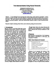
The figures at APPENDIX I (Fig 3. to Fig. 8) show the models outputs scatter plot (observations against estimations) and it is possible to visually confirm that NNCM regression models achieved reasonable effectiveness, even in the case of Abalone experiment. Any other nonlinear regression model could be used in the experiments; however, since the model for pattern recognition depends on the errors produced by the regression models, the methodology may not work properly in cases of regression models with extremely low performance. C. NNCM Regression Models Confidence Intervals The confidence intervals were constructed by adjusting t location-scale distributions to the errors produced by the NNCM regression models with the training datasets, and calculating the values of the inverse cumulative distribution functions for the t distributions, evaluated at the probability α = 90%. TABLE IV shows inferior and superior limits values of the confidence intervals. It is possible to verify that the error distributions were slightly skewed. This information is confirmed, in Fig. 2, that depicts the case of HOUSING experiment where the t location-scale

Fig. 2. HOUSING: error distribution and the adjusted distributions: t location-scale and normal.

TABLE V shows the absolute number and the percentage of the observations located inside of the each one of the confidence intervals. TABLE V NUMBER OF OBSERVATIONS INSIDE OF THE CONFIDENCE INTERVAL FOR = 90% CONFIDENCE LEVEL Experiment Training Dataset Testing Dataset Abalone Concrete EnergyC EnergyH Housing Parkinsons

3444 (89.62%) 861 (90.82%) 630 (89.11%) 631 (89.25%) 411 (88.20%) 4814 (89.07%)

297 (88.92%) 65 (79.27%) 52 (85.25%) 48 (78.69%) 23 (57.50%) 408 (86.81%)

As consequence of calculating the values of the inverse cumulative distribution functions for the adjusted t distributions, evaluated at the probability α = 90%, the percentage of observations, in the training dataset, located inside of the confidence intervals resulted close to 90%. As expected, lower percentage values were achieved in the testing datasets. The confidence interval limits were used to classify the observations in the training dataset according to the definition in Section II, formula (3), and this classification was used to construct the models for the error pattern recognition. D. NNCM Models for Error Pattern Recognition Outcomes All models were implemented in MATLAB with Neural Network Toolbox, Optimization Toolbox, and Statistics Toolbox, and constructed according to the description and following the procedures detailed in Session III.C.

Again, the NNCM models were composed of 20 individual neural networks hidden layer with the number of neurons equal to twice the number of input parameters. Also, all features were selected to be used as input data. The penalty values of the cost matrices were defined after testing different values for the FN penalty, keeping the FP penalty valued fixed in 1. In order to balance the false-positive and false-negative misclassification, in the training datasets, the following criterion was applied: increase the FN penalty, starting from 1.0 with step 0.1, trying to increment the number of classified observation without raising to much the number of false-positive. The FN penalty values defined for each experiment are displayed on TABLE VI.

TABLE VII (CONT.) CONFUSION MATRIX METRICS Experiment

EnergyH

Housing

Parkinsons

TABLE VI FN (FALSE-NEGATIVE) PENALTY VALUE Experiment FN Penalty Abalone Concrete EnergyC EnergyH Housing Parkinsons

1.1 1.5 1.5 1.7 3.0 1.5

As shown in TABLE VII, the experiments confirmed the information mentioned in the literature that, for extremely imbalanced dataset, Sensitivity is often low. This indicates that the models were able to classify only few observations; however, as indicated by reasonable high Precision values, these classifications were correct, in most part of the cases, in training and most importantly, in testing datasets. In other words, the models for pattern recognition datasets were able to identify observations in testing dataset that are more likely to produce higher error values. As expected, all experiments were able to produced high Accuracy and Specificity percentage values denoting good performance in correct classifying the majority class. TABLE VII shows the confusion matrices and the four evaluation metrics (Accuracy, Precision, Specificity, and Sensitivity) of the models in all experiments, for training and testing datasets. TABLE VII - CONFUSION MATRIX METRICS Experiment

Abalone

Concrete

EnergyC

Training Dataset

Testing Dataset

Accuracy: Precision: Specificity: Sensitivity:

90.03% 60.53% 99.13% 11.53%

Accuracy: 89.52% Precision: 62.50% Specificity: 98.99% Sensitivity: 13.51%

Accuracy: Precision: Specificity: Sensitivity:

91.35% 55.10% 97.44% 31.03%

Accuracy: Precision: Specificity: Sensitivity:

92.93% 80.00% 98.46% 23.53%

Training Dataset

Testing Dataset

Accuracy: Precision: Specificity: Sensitivity:

89.39% 53.85% 99.05% 9,21%

Accuracy: Precision: Specificity: Sensitivity:

80.33% 100.00% 100.00% 7.69%

Accuracy: Precision: Specificity: Sensitivity:

91.20% 76.92% 98.54% 36.36%

Accuracy: Precision: Specificity: Sensitivity:

67.50% 83.33% 95.65% 29.41%

Accuracy: Precision: Specificity: Sensitivity:

90.43% 64.92% 98.19% 27.24%

Accuracy: Precision: Specificity: Sensitivity:

88.51% 65.38% 97.79% 27.42%

The figures at APPENDIX II (Fig 9. to Fig. 14) depict similar information in graphic format, showing all error values, the classified observations and confidence interval, in the testing datasets. As noted before, the information about the classified observations can be used for data analyses or decision making, for instance, to assist input data measurement error identification, or just to define observations to be excluded from the testing dataset in order to improve the overall prediction outcome. TABLE VIII summarizes the total effect of the exclusion of the classified observations from the testing dataset. It shows the percentage of improvement in RMSE, R-Squared and Adjusted R-Squared values compared to the values on TABLE III, for all experiments. TABLE VIII VALUES FOR TESTING DATASET AFTER CLASSIFIED OBSERVATIONS EXCLUSION

Experiment

RMSE

R-Squared

Adj R-Square

Abalone Improv.% Concrete Improv.% EnergyC Improv.% EnergyH Improv.% Housing Improv.% Parkinsons Improv.%

1.5374 7.40% 4.2649 11.24% 0.5197 22.94% 0.4086 1.20% 2.6446 21.73% 2.9744 6.59%

0.6240 2.04% 0.9215 0.79% 0.9970 0.10% 0.9987 0.01% 0.9073 4.54% 0.9173 1.30%

0.6229 2.05% 0.9205 0.79% 0.9969 0.10% 0.9987 0.01% 0.9044 4.63% 0.9171 1,30%

V. CONCLUSION Although the percentage of improvement in RMSE, RSquared, and Adjusted-Squared values shown in TABLE VIII seem arguably small, the models for pattern recognition were consistently capable to correctly predict classified observations in testing datasets, accomplishing to yield high Precision and Specificity percentage values. Ultimately, the experiments provided evidence that the methodology presented in this work is able to properly identify observations for which the regression models can

potentially fail, and these individualized indications may be used as an additional assessment to provide better support for tasks like measurement error detection, mistyped data recognition, outlier identification, and general data analysis and investigation. The method only assumes that training and testing datasets follow the same probability distribution, and it can be applied to any kind of regression model with any kind of confidence interval construction method. Regarding the model for error pattern recognition, the key point is the capability of the model of properly handling imbalanced data, because standard classification algorithms tend to misclassify the minority class observations and generate high number of false-positives. Due to this requirement, the methodology would not be recommended for databases with a relatively small number of observations. Further research could evaluate the methodology on different databases, using other kinds of nonlinear regression models, other confidence interval construction methods, and other models for pattern recognition.

Fig. 6. NNCM regression model outcome for EnergyH.

APPENDIX I: REGRESSION MODELS OUTPUTS

Fig. 7. NNCM regression model outcome for Housing.

Fig. 3. NNCM regression model outcome for Abalone.

Fig. 8. NNCM regression model outcome for Parkinsons.

APPENDIX II: TESTING DATASETS ERRORS PLOT

Fig. 4. NNCM regression model outcome for Concrete.

Fig. 9. Abalone: errors plot for testing dataset with confidence interval and classified observations. Fig. 5. NNCM regression model outcome for EnergyC.

Fig. 10. Concrete: errors plot for testing dataset with confidence interval and classified observations.

Fig. 13. Housing: errors plot for testing dataset with confidence interval and classified observations.

Fig. 11. EnergyC: errors plot for testing dataset with confidence interval and classified observations.

Fig. 14. Parkinsons errors plot for testing dataset with confidence interval and classified observations.

REFERENCES [1] [2] [3] [4] [5]

[6]

[7] Fig. 12. EnergyH: errors plot for testing dataset with confidence interval and classified observations.

[8]

[9]

P. McCullagh and J. Nelder, Generalized Linear Models, Chapman & Hall, 1994. W. Enders, Applied Econometric Time Series, John Wiley & Sons, Inc., 2004. J. Wooldridge, Introductory Econometrics: A Modern Approach, 2nd Ed., Thomson South-Western, 2003. Bates, D. M., and Watts, D. G. – “Nonlinear regression analysis and its applications” - New York: Wiley, 1998. G. Papadopoulos, P.J. Edwards, A.F. Murray, “Confidence Estimation Methods for Neural Networks: A Practical Comparison” - ESANN’ 2000 procedings, Bruges(Belgium), April/2000. R. Polikar – “Bootstrap-Inspired Technique in Computational Intelligence” - IEEE SIGNAL IEEE Signal Processing Magazine, 59, May/2007. C.P.Hinsbergen, J.Lint, H. Zuulen - “Bayesian committee of neural networks to predict travel times with confidence intervals” – Science Direct, 2009. A. Khosravi and S. Nahavandi, “Lower Upper Bound Estimation Method for Construction of Neural Network-Based Prediction Intervals” - IEEE Transaction on Neural Networks, Vol. 22, No. 3, March 2011. H. Quan, D. Srinivasan and A. Khosravi, “Construction of Neural Network-based Prediction Intervals using Particle Swarm Optimization” – WCCI 2012 IEEE World Congress on Computational Intelligence, 10-15, June, 2012.

[10] H. Papadopoulos – “Inductive Conformal Prediction: Theory and Application to Neural Networks”, InTechOpen, August, 2008. [11] H. Papadopoulos and H. Haralambous – “Reliable prediction intervals with regression neural networks” – Neural Networks 24, 842-851, Elsevier, 2011. [12] J. N. Warwick, T. L. Sellers, S. R. Talbot, A. J. Cawthorn and W. B. Ford - "The Population Biology of Abalone (Haliotis species) in Tasmania. I. Blacklip Abalone (H. rubra) from the North Coast and Islands of Bass Strait" - Sea Fisheries Division, Technical Report No. 48 (ISSN 1034-3288), 1994. [13] Y. I-Cheng, "Modeling of strength of high performance concrete using artificial neural networks" , Cement and Concrete Research, Vol. 28, No. 12, pp. 1797-1808, 1998. [14] A. Tsanas and A. Xifara – “Accurate quantitative estimation of energy performance of residential buildings using statistical machine learning tools” - Energy and Buildings, Vol. 49, pp. 560-567, 2012. [15] D. Harrison, and D.L.Rubinfeld, “Hedonic prices and the demand for clean air”, J. Environ. Economics & Management, vol.5, 81-102, 1978. [16] T.Athanasios, A.L. Max, E.M. Patrick, and O.R. Lorraine, “Accurate telemonitoring of Parkinson.s disease progression by non-invasive speech tests”, IEEE Transactions on Biomedical Engineering 2009. [17] G.H. Nugye, A. Bouzerdoum and S.L. Phung, Learning Pattern Classification Tasks with Imbalanced Data Sets, Pattern Recognition Peng-Yeng Yin (Ed.), 2009. [18] S. Kotsiantis, D. Kanellopoulos and P. Pintelas – “Handling imbalanced datasets: A Review” – GESTS International Transactions on Computer Science and Engineering, Vol. 30, 2006. [19] Z.H. Zhou, J.Wu and W.Tang – “Ensembling neural networks: Many could be better than all” – Science Direct, 2001. [20] G. Basawaraj, K. Subhash, B. Chandrasekhar , “Novel Ensemble Neural Network Models for better Prediction using Variable Input Approach” – International Journal of Computer Applications (0975 – 8887) Volume 39– No.18, February 2012. [21] E. Mazloumi, G. Rose, G. Currie, S. Moridpour - “Prediction intervals to account for uncertainties in neural network predictions: Methodology and application in bus travel time prediction” – Elsevier, 2011. [22] S. Haykin, Neural Network and Learning Machines (3rd Edition), Pearson Education, Inc. 2009. [23] S. Samarasinghe, Neural Networks for Applied Sciences and Engineering: From Fundamentals to Complex Pattern Recognition, Auerbach Publications, 2007. [24] A.M.S.Yaser, I.M.Magdon, H.T.Lin, Learning From Data, AMLBook, 2012. [25] R. Duda, D. Stork, P. Hart, Pattern Classification – John Wiley & Sons (2005).