tracking single moving limb in a color image sequences. In our method the normal flow is computed directly from color images and used for both limb detection ...
Using Normal Flow for Detection and Tracking of Limbs in Color Images Zoran Duric, Fayin Li, Yan Sun, Harry Wechsler Department of Computer Science George Mason University Fairfax, VA 22030 {zduric,fli,ysun,wechsler}@cs.gmu.edu Abstract Humans are articulated objects composed of non-rigid parts. We are interested in detecting and tracking human motions over various periods of time. In this paper we describe a method of detecting and tracking human body parts in color video sequences. The dominant motion region is detected using normal flow; Expectation Maximization, uniform sampling, and a shortest path algorithm are used to find the bounding contour for the moving arm. An affine motion model is fit to the arm region; residual analysis and outlier rejection are used for robust parameter estimation. The estimated parameters are used for the prediction of the location of the moving limb in the next frame. Detection and tracking results are combined to account for the deviations from the affine flow model and increase the robustness of the method. We demonstrate our method on several long image sequences corresponding to different limb movements.
1. Introduction Humans are articulated objects composed of non-rigid parts. We are interested in describing and recognizing their motions over various periods of time. Recent reviews on machine analysis of human motions by Gavrila [3], Aggarwal and Cai [1], and Moeslund and Granum [5] provide excellent coverage of research on detection and tracking of human motions. It is widely accepted that automatic detection of nonrigid moving objects and their accurate tracking in long image sequences still remain very challenging. In this paper we address the problem of detecting and tracking single moving limb in a color image sequences. In our method the normal flow is computed directly from color images and used for both limb detection and tracking. A shortest path algorithm is used to link detected edges and delineate the contour of the moving limb. Affine flow model is fit to the computed flow to predict the position of the limb in the next frame. The estimated affine flow is compared to
the computed normal flow to obtain the residuals. A residual analysis is performed and outliers are rejected; affine motion parameters are reestimated for the remaining flow vectors. The computed affine parameters are used to predict the position of the arm in the next frame. The predicted position is combined with the results of detection to account for model inaccuracies and nonrigidity of the moving limb. In the remainder of the paper we describe our method and present the results of limb detection and tracking on color image sequences. In Section 2 we address the motion estimation issues. In Section 3 we present some experimental results and in Section 4 we present the conclusions and discuss future work.
2. Limb Detection and Tracking In Section 2.1 we describe how we estimate normal flow in color images. In Section 2.2 we describe how we detect and outline moving limbs. In Section 2.3 we describe how we estimate affine flow model from normal flow. In Section 2.4 we describe our method of tracking moving limbs.
2.1. Normal Flow Estimation In this section we briefly describe our method of computing normal flow in color images; the details of the method will be reported elsewhere. We first describe our algorithm for computing normal flow in gray level images. Let ~ı and ~ be the unit vectors in the x and y directions, respectively; δ~r = ~ıδx + ~δy is the projected displacement field at the point ~r = x~ı + y~. If we choose a unit direction vector ~nr = nx~ı + ny~ at the image point ~r and call it the normal direction, then the normal displacement field at ~r is δ~rn = (δ~r · ~nr )~nr = (nx δx + ny δy)~nr . ~nr can be chosen in various ways; the usual choice (and the one that we use) is the direction of the image intensity gradient ~nr = ∇I/k∇Ik. Note that the normal displacement field along an edge is orthogonal to the edge direction. Thus, if at time t we
observe an edge element at position ~r, the apparent position of that edge element at time t + ∆t will be ~r + ∆tδ~rn . This is a consequence of the well-known aperture problem. We base our method of estimating the normal displacement field on this observation. For an image frame (say collected at time t) we find edges using an implementation of the Canny edge detector. For each edge element, say at ~r, we resample the image locally to obtain a small window with its rows parallel to the image gradient direction ~nr = ∇I/k∇Ik. For the next image frame (collected at time t0 + ∆t) we create a larger window, typically twice as large as the maximum expected value of the magnitude of the normal displacement field. We then slide the first (smaller) window along the second (larger) window and compute the difference between the image intensities. The zero of the resulting function is at distance un from the origin of the second window; note that the image gradient in the second window at the positions close to un must be positive. Our estimate of the normal displacement field is then −un , and we call it the normal flow. In color images (RGB) we apply an edge detector to each color band to obtain partial derivatives rx , ry , gx , gy , bx , by for the (r)ed, (g)reen, and (b)lue bands. Edges in color images can be computed using a standard technique used for processing multi-channel imagery [4]. We first form a matrix S, � � rx ry + gx gy + bx by rx2 + gx2 + b2x . S= rx ry + gx gy + bx by ry2 + gy2 + b2y The trace of S corresponds to the edge strength. If there is an edge at point (x, y), the larger eigenvalue of S, λ1 , corresponds to the edge strength. The corresponding eigenvector (nx , ny ) represents the edge direction. Therefore we can treat color edges in the same manner as we have treated gray level edges. The only difference is that the edge strength and the edge direction correspond to the larger eigenvalue of S and its corresponding eigenvector. For each edge element, say at ~r, we resample the three image color bands locally to obtain three small windows with their rows parallel to the image gradient direction ~nr = (nx , ny ). For the next image frame (collected at time t0 + ∆t) we create a larger window, typically twice as large as the maximum expected value of the magnitude of the normal displacement field. We then slide the first (smaller) window along the second (larger) window and compute the difference between the image intensities in all three color bands. The result is a vector function (δr , δg , δb ) of the color differences. The magnitude of this vector has a zero crossing at distance un from the origin of the second window; the difference vector changes sign around the zero crossing. We estimate the zero crossing by comparing the magnitudes of the two difference vectors pointing in opposite directions.
350
300
250
200
150
100
50
0
50
100
150
200
250
300
350
Figure 1. The first frame from a color image sequence of 400 frames and its corresponding normal flow. These images were collected using a Sony DFW-VL500 progressive color scan camera; the frame rate was thirty frames per second and the resolution was 320 × 240 pixels per frame.
Our estimate of the normal displacement field is then −un , and we call it the normal flow. Figure 1 show an example of normal flow computed for the first frame of an image sequence. The arm motion is nonrigid because of the loose clothing.
2.2. Moving Limb Detection and Delineation In a typical image the background is larger than the foreground and most background edges do not move; note that the shadows move. However, due to various factors including camera noise, shadows, and lightning variations between frames 1 the normal flow in the background is nonzero. In addition, the foreground edges usually have larger motion than the background edges, but due to interaction of the background and the foreground (“T-junctions”) we cannot compute flow everywhere and at some points computed values are not reliable. To separate the foreground and the background edges, we assume that the the normal flow values (projections on the image gradients) in the background have a Gaussian distribution. We use the Expectation Maximization (EM) [6] to fit a Gaussian to the histogram of normal flow values. We assume that the normal flow values < 4σ belong to the background and that the normal flow values ≥ 4σ belong to the foreground; we use 4σ threshold to reduce noise in the foreground detection. We compute a bounding box for the parts of the image that have normal flow values higher than the 4σ threshold. We scan the inside of the box to find the outside layer of the points within the box. We select points which have large values of the gradient as well as large normal flow values. We choose sample points from the selected points based on similarity of their gradient and flow values with their neighbors. The sample points are linked to their neighbors using 1 We rely on normal ambient lights that correspond to a mixture of neon light panels and outdoor lights.
equation ai · u ≈ un,i . Let the number of edge points be N ≥ 6. We then have a system Au − b = E where u is an N -element array with elements un,i , A is an N × 6 matrix with rows ai , and E is an N -element error vector. We seek u that minimizes kEk = kb−Auk; the solution satisfies the system AT Au = AT b and corresponds to the linear least squares solution.
2.4. Limb Tracking
Figure 2. Delineating the foreground objects for images in Figure 1. Upper row: points with high normal flow values and high gradient magnitudes. Lower row: foreground object outlines.
a variation of the Dijkstra’s shortest path algorithm [2] to create a connected contour. The cost of the path is obtained by subtracting the gradient magnitude value from the maximum gradient magnitude computed for the image. Figure 2 shows the selected points and the computed contours for images in Figure 1.
2.3. Estimating Affine Motion Parameters Let (x, y) be the image coordinates of a pixel in an image I(x, y) and let the image be centered at (0, 0). We have the following expression for the affine displacement (δx, δy) of the point (x, y) due � � � �� � � � δx a b x e = + . (1) δy c d y f Using Equation (1) we obtain the normal displacement field at (x, y) as δ~rn · ~nr = nx δx + ny δy = anx x + bnx y + enx + cny x + dnx y + f ny ≡ a·u (2) where ~nr = nx~ı + ny~ is the gradient direction at (x, y), a = (nx x nx y nx ny x ny y ny )T , and u = (a b e c d f )T is the vector of affine parameters. We use the method described in Section 2.1 to compute normal flow. For each edge point ~ri we have one normal flow value un,i which we use as the estimate of the normal displacement at the point. This gives us one approximate
We delineate a moving arm for a given frame using the method described in Section 2.2. We use all image points with high gradient values within or on the detected contour to estimate the affine flow parameters for that frame. We subtract the normal flow from the normal motion field given by the affine parameters to compute the residual normal flow field. We observe that the residual normal flow values should be small and that their distribution should be similar to the distribution of the background normal flow values. However, due to various factors including noise, shadows, lightning variations, and interactions of the background with the foreground, we expect to have residual values corresponding to outliers. We use the same EM method as in Section 2.2 to estimate the Gaussian distribution and detect the outliers. After the outlier detection and rejection we reestimate the affine motion parameters by using the remaining normal flow vectors; the second estimate is usually much better than the first one. Figure 3 shows examples of the residual flow fields and the reestimated affine flows for the detected arms in 2. After outlier rejection and affine parameter reestimation, we use the computed affine motion parameters to predict the position of the arm in the next frame. The position of the point in the current frame plus its estimated affine flow are used to predict its position in the next frame. Note that we only use those points in the current frame that have small residuals; we assume that points with large flow residuals are erroneous. We vary the affine parameters in a small range to obtain multiple candidate points in the next frame; this is used to help account for errors in the model (e.g., the shirt moves nonrigidly) and in the parameter estimation. From the candidate points in the next frame, we select those points that have the largest motion and/or gradient magnitude values in their neighborhoods. At the same time, we perform moving object detection in the manner described in Section 2.2 to detect all points that have large motions. These points are added to the tracked points from the previous frame. From these points we sample uniformly and link the neighbors by a shortest path algorithm; the neighbors are determined with respect to the points corresponding to them in the previous frame. Using this method we
210
180
200 160 190
180 140 170
160
120
150 100 140
130 80 120
110
0
50
100
150
200
250
60
240
180
220
160
200
140
180
120
160
100
140
80
120
100
0
50
100
150
200
250
Figure 4. Frames 50, 101, 155, and 198 from the “pounding” sequence. Top row: color frames. Lower row: tracked contours.
60
0
50
100
150
200
250
40 −50
0
50
100
150
200
250
Figure 3. Residual and reestimated flows for the detected arms in Figure 2. Upper row: residual flow computed as the difference between the computed normal flow and the estimated affine normal motion field. Lower row: reestimated affine flow after outlier rejection.
have been able to fully automate detection and tracking of moving limbs in long image sequences.
3. Experimental Results In this section we demonstrate our method on two long color image sequences. The first sequence of 400 frames corresponds to pounding (up, down) motion. The second sequence of 100 frames corresponds to swirling (circle) motion. These images were collected at our laboratory using a Sony DFW-VL500 progressive color scan camera; the frame rate was thirty frames per second and the resolution was 320 × 240 pixels per frame. The moving arm was detected and tracked automatically using the methods described in Section 2. Figure 4 shows 4 frames and the corresponding tracked contours for the “pounding” sequence. Figure 5 shows 4 frames and their corresponding tracked contours from the “swirling” sequence.
4. Conclusions We have described a normal flow based method of detection and tracking of limbs in color video sequences. The moving limb is detected automatically, without manual initialization, foreground or background modeling. An affine motion model is fit to the arm region and the estimated parameters are used for the prediction of the location of the moving limb in the next frame. The predicted location is
Figure 5. Frames 3, 22, 32, and 53 from the “swirling” sequence. First row: color frames. Second row: tracked contours.
combined with the detection results to fit the “best” contour to the moving limb. We have demonstrated our results on color sequences of moving hands. Future work includes automatic detection and tracking of articulated motions.
References [1] J. Aggarwal Q. Cai. Human motion analysis: A review. Computer Vision and Image Understanding, 73:428–440, 1999. [2] T.H. Cormen, C.E. Leiserson, and R.L. Rivest. Introduction to Algorithms. The MIT Press, Cambridge, Massachusetts, 1990. [3] D.M. Gavrila. The visual analysis of human movement: A survey. Computer Vision and Image Understanding, 73:82– 98, 1999. [4] B. J¨ahne. Digital Image Processing. Springer-Verlag, Berlin, Germany, 1997. [5] T.B. Moeslund and E. Granum. A survey of computer visionbased human motion capture. Computer Vision and Image Understanding, 81:231–268, 2001. [6] W. Oh and W.B. Lindquist. Image thresholding by indicator kriging. IEEE Trans. on Pattern Analysis and Machine Intelligence, 21:590–602, 1999.