Handbook of Mathematical Functions continues to be widely used by the ... the DLMF will be 3D graphics and visualization capabilities that allow a user to ...
Using Numerical Grid Generation to Facilitate 3D Visualization of Complicated Mathematical Functions Bonita Saunders, Qiming Wang
Abstract Although virtually unchanged since its initial publication in 1964, the National Bureau of Standards (NBS) Handbook of Mathematical Functions continues to be widely used by the mathematical and scientific community. As a result, the National Institute of Standards and Technology (NIST), the successor organization to NBS, is engaged in a large scale project to update and expand the handbook and disseminate it on the World Wide Web as the NIST Digital Library of Mathematical Functions (DLMF). A key feature of the DLMF will be 3D graphics and visualization capabilities that allow a user to interactively examine the unique features of complicated mathematical functions. The authors have discovered that many commercial packages produce adequate surface plots of functions, but improperly clip the surface when the plot must be rescaled to emphasize interesting features. This paper discusses some initial results in using a “contour” fitted mesh to generate an appropriately clipped surface plot and examines some of the issues involved in extending the technique to more complicated surfaces. Keywords: grid generation, 3D clipping, special functions, scientific visualization, virtual reality modeling language
1
Introduction
• advances in basic mathematical and computational techniques associated with the classical special functions of the mathematical and physical sciences; and
The Handbook of Mathematical Functions [1] is a well known publication of the National Bureau of Standards, the predecessor organization of the Na• the identification of new functions having tional Institute of Standards and Technology (NIST). widespread importance in emerging applicaAlthough there have been no major revisions since its tions initial publication in 1964, it continues to be widely sold by the US Government Printing Office, Dover, have led NIST to embark on a massive project to and many other commercial publishers. The contin- update and expand the current handbook and disued interest in the handbook plus such factors as seminate it in digital format on the World Wide Web; see Lozier [2] for an early description and • the clear advantages of electronic media for http://dlmf.nist.gov/ for current information on the construction and communication of ideas this new project. The new entity, which is being called the Digital Library of Mathematical in technical fields;
1
Functions (DLMF), will make full use of advanced communications and computational resources. A key feature of the DLMF will be dynamic 3D visualizations of special functions that allow a user to conduct interactive explorations of the relationship between a function’s mathematical or numerical properties and its graphical representations.
Language) format. VRML [3] is a standard 3D file format for describing the behavior and geometry of a 3D virtual world, or scene. Its accessibility on the Internet and interactive capabilities make it an ideal candidate for this development work. Since all aspects of the DLMF will be designed to be accessible to as large an audience as possible, users must not be required to purchase proprietary software in order to use any of its features. VRML browser plugins are available by free download for a variety of platforms. Still, it is not a foregone conclusion that the final version of the DLMF will use VRML. This may depend on whether VRML browsers continue to be readily available. Also, we are looking at alternatives to VRML such as JAVA 3D which would not require the download of a browser, but still would require the user to obtain the graphics package. In our mockup DLMF we give the user the option of viewing a still 3D image if a VRML browser is not available.
While constructing 3D graphical representations for a sample chapter of a mockup version of the DLMF, the authors discovered that problems may arise when graphs must be rescaled to emphasize peaks, zeros, poles and other interesting features. Many packages fail to clip the surfaces properly. Some produce ragged uneven edges and others create a misleading “shelf” effect. To address this problem, the authors are studying the feasibility of obtaining clipped surfaces by computing complicated mathematical functions over “contour fitted” meshes. This paper examines the clipping problem, looks at some of the results obtained to date for the prototype chapter, and offers Figure 1 shows a VRML display from the prototype some suggestions on what might be done for multi- chapter on Airy functions in our mockup Web site. connected and more complicated domains. The Airy functions, Ai and Bi, occur in quantum mechanics, in the study of wave diffraction, electromagnetism, and other areas of physics and engineering, 2 3D Visualization in a Web- and arise as solutions of the second order differential equation Based Digital Library d2 w = zw dz 2 Like the original handbook, the DLMF is designed primarily for the use of scientists. A secondary, but where z is complex. The display shows |Ai(z)|. The important goal is to reach a much broader audience browser controls allow the user to rotate the figure, by making aspects of the DLMF accessible to educa- zoom in and out, and move the figure in an arbitrary tors and students. An obvious way to support these direction. dual goals is to create 3D visualizations that are both exciting and informative. Fortunately, the graphical representations of many special functions are so complex and interesting that by designing visualizations that illustrate the features of interest to scientists we automatically produce displays that grab the attention of less technically oriented viewers.
2.1
Static and Dynamic Visualizations of Special Functions
For both the still images and interactive visualizations in the DLMF we begin with a preprocessing stage, using available packages such as MATLAB and MATHEMATICA to plot the data so that we can examine the graphical representation and adjust the scaling to bring out interesting features. While the still images are stored in GIF or POSTSCRIPT format, dynamic visualizations are obtained by converting the data to VRML (Virtual Reality Modeling
Figure 1: VRML display on CosmoPlayer.
2
The preprocessing of the data mentioned earlier is necessary because VRML is not designed to do extensive computations. Therefore, any adjustments to the range, rescaling, and clipping are done before the data is transformed to VRML format. However, VRML does allow one to add custom designed features to the browser. One such feature we have added is a cutting plane control panel which gives the user the capability to generate cutting planes through the surface. By clicking on the buttons on the control panel the user can move the plane in sync with the projected intersection curve, displayed on opposite faces of the bounding box as shown in Figure 2. Computing a surface over a structured grid nicely orders the data points so that it is easier to design efficient software that computes the intersection of the surface with a plane.
the plotting range. In such a case the surface should be clipped so that the outside points do not appear. Commercial packages handle this situation in a variety of ways. MATLAB performs 2D clipping well, but has problems with 3D clipping. In some cases it does not clip the surface at all, allowing it to extend beyond the plotting range. MATHEMATICA clips in a variety of ways depending on whether you use Graphics3D, SurfaceGraphics, or the extra ExtendGraphics packages [4]. SurfaceGraphics is designed for surfaces that do not fold over, while Graphics3D can be used to represent any 3D object. In both cases the default method of clipping is to reset values outside the plotting range to the same constant. This produces the misleading shelf effect seen in the plot of |Bi(z)| over an equally spaced rectangular domain in Figure 3. This technique is extensively used by William J. Thompson in Atlas for Computing Mathematical Functions [5]. The user has the 1
mathshelf.nb
5 4 4 3 2 2 1 0 0 -2 -2 0
Figure 2: VRML display with Y direction cutting plane.
2.2
2
Out[1]=
3D Clipping
-4
SurfaceGraphics
Figure 3: Clipped version of |Bi(z)| using Mathematica.
In general, commercial packages, such as MATLAB and MATHEMATICA, produce a default scaling of a surface that is designed to give the best overall view. However, when the function values vary widely over the plotting domain, the default view may fail to show interesting features such as zeros, poles, or saddle points. In many cases adjusting the plotting domain and rescaling the graph may be enough to emphasize points of interest and produce an aesthetically pleasing plot. This was true for most of the graphs designed for our sample chapter on Airy functions in the mockup DLMF. However, sometimes rescaling the graph may cause some points to fall outside
option of leaving out the clipped areas, but that produces jagged edges that are equally misleading as seen in Figure 4. By resetting the plotting range after drawing the surface, we obtained the smoothly clipped surface in Figure 5 using Graphics3D, but not SurfaceGraphics. A similar result can be obtained by using the Clip3D routine in the ExtendGraphics package. Although the clipped surface looks very good, Figure 6 shows that when the data is converted to VRML format the 3
2
mathshelf.nb
2
mathclip2.nb
5 4 4
3
5
2
4
2
4
1
3
0 2
0
2 1 -2 0 -2
0 0 -2 2
-2
-4
0
Out[4]= 2
Out[2]=
Graphics3D
-4
SurfaceGraphics
Figure 4: Clipped version of |Bi(z)| with shelf deleted. Figure 5: Clipped version of |Bi(z)| using Mathematica Graphics3D object. shading appears unsmooth with harsh shadows. The surface shading is based on the height of the surface at that grid point. The grid lines in Figure 4 rise at sharp angles toward the top of the surface. When the data is converted to VRML, the scaling used makes the angles even sharper. If the grid lines were shown on the VRML surface, one would see that the colors associated with the grid points change quickly as one traces a grid line to the top of the surface. This is probably the reason for the “ugly” shading. We will show that plotting the function over our contour fitted grid decreases this problem significantly.
eral holes where poles are located. Other functions have zeros whose exact locations must be plotted, or a domain of disconnected parts. Still others may have a combination of complicated features. It is clear that the grid generation problem may be quite simple or extremely complex. Hence, it would be difficult to design techniques that cover all situations. In this section we describe the technique used to clip surfaces in the prototype chapter and discuss the results obtained.
3.1
3
Contour Fitted Grid Generation
Technique
The first step is to determine what features should be emphasized and what plotting range and domain size are needed to bring out the features. For the DLMF this may actually be a very time consuming process, requiring close collaboration with the author of the chapter for which the visualizations are being designed. The authors of the DLMF will be world renowned specialists in the field of special functions located both inside and outside the US. Most communication will have to be done electronically, but it is expected that at some point the authors will spend some time at NIST working on the project.
The basic idea behind 3D visualization using contour fitted grid generation is to compute the function over a grid bounded by a contour of the function rather than over a uniform rectangular grid. The idea is simple, but the ease or difficulty of implementing the technique depends on several factors. The contour map of the function may be very complex. In general, contours representing the same height may not be connected. Therefore a decision has to be made as to the best way to connect the curves so that a conThe next step is to compute a contour map of the tinuous boundary is formed. Also, the domain may function based on the endpoints of the plotting range be quite complicated. For example, the domain of the chosen. A continuous outer boundary and interior gamma function in the complex plane contains sevboundaries, if necessary, are then designed with the
4
1000
800
Z
600
400
200
0 1.5 1
5
0.5
0
0
−5 −0.5
−10 −1
Y
Figure 6: VRML display of |Bi(z)| using Mathematica data.
−20
X
Figure 7: Default plot of |Bi0 (z)| using MATLAB.
function. After the contours were connected to the
contour curves as the major components. At this point the problem is choosing a method to generate a boundary fitted grid. For extremely complicated domains, an unstructured method may be required, but for simpler domains, structured methods are desirable. The reason is that nicely ordered grid lines will produce a smoothly shaded surface when the VRML conversion is done. Also, with structured grids more efficient code can be designed for the computation and movement of cutting planes. The next section examines the specific results obtained for the sample chapter.
3
2
1
0
−1
−2
−3 −4
3.2
−15 −1.5
Results
−3
−2
−1
0
1
2
Figure 8: Contour curves where Z=5.
Fortunately, in the sample chapter developed for the mockup DLMF only Airy functions |Bi(z)| and |Bi0 (z)| needed clipping. Suitable plots of the other ten surfaces were obtained by adjusting the plotting range and size of the rectangular computational domain. Since the contour map and features of the two functions are quite similar, only the results for |Bi0 (z)| are discussed. Figure 7 shows a plot of |Bi0 (z)| with the default plotting range selected by MATLAB. The range is so large that the key features of the function are essentially damped out. After conferring with the author of the Airy function chapter and experimenting with various plotting ranges and mesh sizes, it was determined that a plotting range of 0 ≤ Z ≤ 5 was sufficient if the computational mesh was restricted to −4.5 ≤ X ≤ 2.5,−3.5 ≤ Y ≤ 3.5. Figure 8 shows the Z = 5 contour curves for the
5
sides of a rectangle to form a continuous boundary, a simple transfinite interpolation map was used to create the boundary fitted mesh shown in Figure 9. Although computing |Bi0 (z)| over the mesh would produce a smoothly clipped surface, there would still be no guarantee that the zeros of the function would fall on the grid lines. On the contour fitted domain |Bi0 (z)| has two real zeros and two complex conjugate pairs of zeros. The transfinite mapping would map some point on the square to each zero location, but determining which points is not a simple task. One possibility would be to design a routine that searches for the grid cell containing the zero and then use interpolation to construct grid lines through the point. Instead, a more exact technique was used. After drawing rough curves through the zeros, cardinal spline blending functions [6]were used
4
clipped by setting all points outside the plotting range equal to 5, thus producing the shelf effect discussed earlier. The surface suffers from the same angled grid line problem seen in Figures 5 and 6 for |Bi(z)|, producing non-smooth shading near the top of the surface. Figure 12 was computed over the contour fitted mesh in Figure 10. The surface is smoothly clipped at Z = 5. The sharp cusps show that grid lines accurately intersect the zeros. Also, the shading is much smoother than what is seen in Figure 11, or even in the clipped surface from Mathematica data shown in Figure 6. This is probably because parts of the grid lines roughly look like contours. Consequently, one would expect that the projection of the grid onto the surface would not show sharply angled grid lines.
3
2
1
0
-1
-2
-3
-4 -5
-4
-3
-2
-1
0
1
2
3
Figure 9: Contour mesh.
to construct a transfinite mapping that interpolates not only the outer contour boundary, but also the curves that pass through the zeros. Using this technique one can choose which points on the square will be mapped to a particular zero. Figure 10 shows the contour mesh obtained with this mapping. An advantage of using a transfinite mapping is that the number of meshpoints can be easily decreased or increased by changing the number of points evaluated on the square. The only requirement is that the mapping always include an evaluation at points known to map to zeros. Of course this may effect the smoothness of the grid as seen in Figure 10, but for this application grid smoothness is not as critical as it would be for a grid being used to compute the numerical solution of Figure 11: |Bi0 (z)|, Modulus of the derivative of partial differential equations. Bi(z). 4
3
2
1
0
-1
-2
-3
-4 -5
-4
-3
-2
-1
0
1
2
3
Figure 10: Contour mesh with extra interpolated curves.
Figures 11 and 12 show the effectiveness of the techFigure 12: Clipped version of |Bi0 (z)|. nique. In Figure 11, |Bi0 (z)| was computed over an equally spaced rectangular domain. The sharp cusps were obtained by adding extra grid lines that intersected the zeros of the function. The surface was Figure 13 shows a view of the clipped surface from 6
4
the top. The darkened circles show the locations of the zeros. Figure 14 shows a cutting plane moving
Conclusions
The use of contour fitted meshes appears to be an effective technique for generating appropriately clipped surface plots. The development of clear and informative 3D visualizations for the NIST DLMF project will provide us with continued opportunities and motivation to explore the clipping problem. Also, after looking at off-the-shelf packages, it appears that research in this area would be of interest to commercial developers of 3D graphics packages. The problem is clearly a complex one, since the domains of complicated functions can vary from the very simple to multi-connected domains with holes. This makes it difficult to design techniques that work for all cases. Somewhat simple structured grids sufficed for the functions in the sample chapter, but more than likely unstructured grids will be needed when we move on to more complex domains.
Figure 13: Top view of clipped |Bi0 (z)|. through |Bi0 (z)| in the X direction. Currently, the mockup Web site only allows the display of cutting planes in the X or Y direction, but work is in progress on the development of more general software allowing cutting planes perpendicular to all coordinate directions.
For the particular case of the DLMF project, the work is further complicated because close collaboration is required between DLMF project members designing and implementing the visualizations and the authors of the DLMF chapters in order to determine the proper plotting range and the locations of zeros, poles, saddle points and other features that should be emphasized. Each chapter will produce new challenges, but the hope is that much of what we are learning now can be easily applied to creating suitable visualizations for the other chapters.
Disclaimer Identification of commercial products in this paper does not imply recommendation or endorsement by NIST.
References [1] M. Abramowitz and I.A. Stegun, editors. Handbook of Mathematical Functions with Formulas, Graphs and Mathematical Tables, Vol. 55, National Bureau of Standards Applied Mathematics Series. U.S. Government Printing Office, Washington, D.C., 1964.
Figure 14: VRML display with X direction cutting plane.
Although we were able to use simple structured grids for our functions, unstructured or multi-block grids may be needed for complex multi-connected domains. Also, whenever possible we want to use available packages. A package may produce an unsatisfactory clipping of one function, but produce an acceptable one of another.
[2] D.W. Lozier, “Toward a Revised NBS Handbook of Mathematical Functions,” NISTIR 6072, National Institute of Standards and Technology, September 1997.
7
[3] VRML. The Virtual Reality Modeling Language, International Standard ISO/IEC 147721:1997. [4] T. Wickham-Jones, Mathematica Graphics, Springer-Verlag, New York, 1994. [5] W.J. Thompson, Atlas for Computing Mathematical Functions, John Wiley and Sons, Inc., New York, 1997, pp. 414-432. [6] G. Birkhoff, C. de Boor, “Error Bounds for Spline Interpolation,” Journal of Mathematics and Mechanics, Vol. 13, No. 5 (1964), pp. 827835.
8